Non-Destructive Inspection
General Description
The Non-Destructive Inspection component is a collection of software tools related to computer vision analysis. The Non-Destructive Inspection - Computer Vision Suite spans from traditional techniques to contemporary innovation, while embracing the design-time and the run-time concepts. This opens the possibility of designing complex computer vision algorithms exploiting image processing techniques and tools and deploying them to a production line.
The Non-Destructive Inspection - Computer Vision Suite is made of:
Runtime: It is an engine that executes computer vision algorithms. This is the core component of the suite, which is why all the other components integrate with the Runtime to execute their functions
Builder: The Non-Destructive Inspection component is not a static collection of algorithms; in fact, it is the opposite. The Runtime works with modules, which are collections of computer vision functions. These modules can be developed, sold, and bought from the Marketplace, and installed though the Builder component. This allows the suite to be quickly extended when new computer vision techniques or algorithms are conceived
Designer: intuitive, web-based UI to compose an algorithm using building blocks. These building blocks are derived from the installed modules just described, and they can be connected to create a flow. These flows can be saved and run through the Runtime. The Designer has a set of debugging tools to quickly develop and debug these flows
AI Image Classifier: web-based UI to solve the classification problem: the categorization of images into one or more classes. It allows users to label images into desired classes and train an AI-model that learns how to classify those images
AI Image Labeller: web-based UI to solve the object detection problem, so as also to address defect detection: the presence, location, and classification of objects in images. This tool contains a complete labelling tool, to quickly tag images, and an AI engine to train a model
Module Creator: developers can create new modules (algorithms) by using this tool
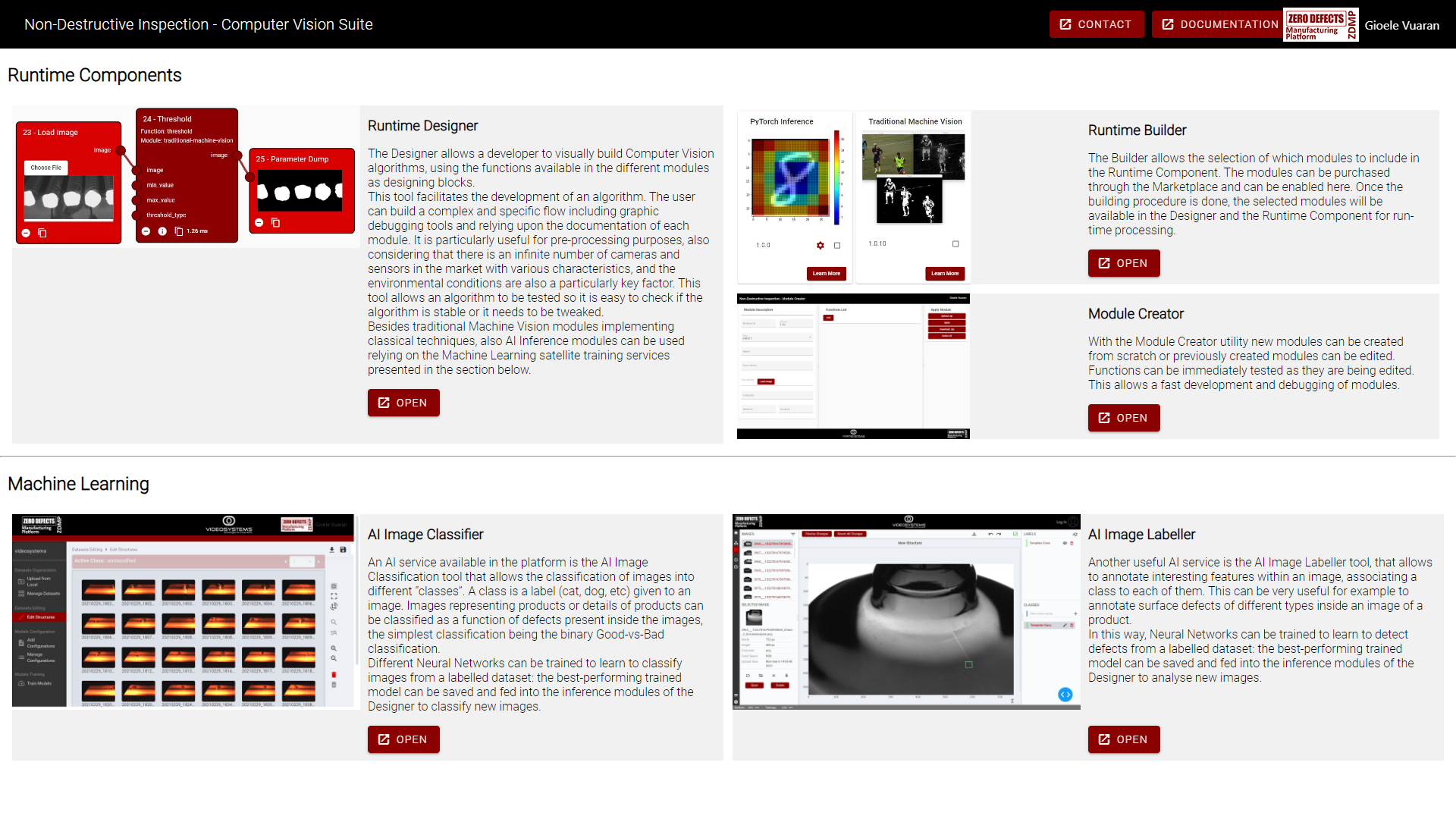 Figure 1. Computer Vision Suite
| Resource | Location |
|---|---|
| Online documentation | Link |
| Open API Spec | Link |
| Video | NDI - Computer Vision Designer and Runtime |
| Related Datasets and Examples | Link |
Screenshots
The following images are illustrative screenshots of the component.
Figure 2. Designer
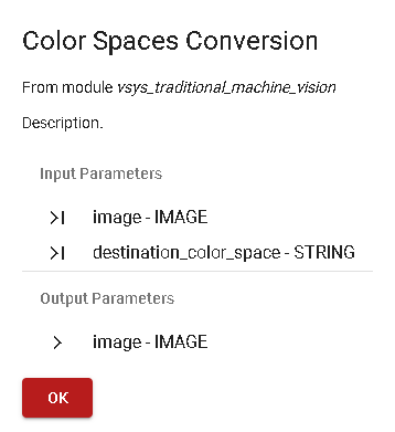
Figure 3. Functions Documentation
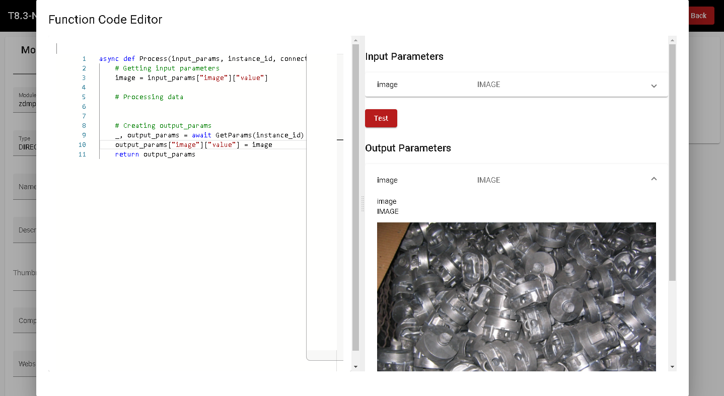
Figure 4. Module Development: Code Editor
Component Author(s)
| Company Name | ZDMP Acronym | Website | Logo |
|---|---|---|---|
| Video Systems Srl. | VSYS | videosystems.it |  |
Commercial Information
| Resource | Location |
|---|---|
| IPR Link | |
| Marketplace product description |
Architecture Diagram
The following diagram shows the position of this component in the ZDMP architecture.
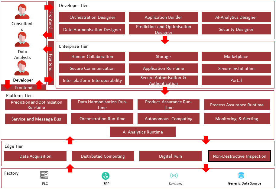
Figure 5. Position of component in ZDMP Architecture
Benefits
Easy development of complex Computer Vision algorithms
Visual debugging tools for easier development and testing
Modular approach to have flexible, extensible, and optimized functionalities
Easy implementation of complex Deep Learning / Neural Networks models
Real-time and historical processing of images
Computer Vision solutions:
Quality Control
Object Recognition
Defects Detection
Metrology
Biometrics
Image Classification
Counting / Presence of an object
Optical Character Reader (OCR) recognition
Barcode / QR / Data Matrix code scanning
Thermal Imaging
Robot guidance (using 3D sensors for the world mapping)
Space Analysis with the help of a robot (robot-mounted 3D sensors)
Robot picking (wall- or robot- mounted 3D or 2D sensors)
Robot Object Recognition and Quality Control
Features
There are many Computer Vision algorithms that use different techniques, for example traditional Machine Vision, Image Processing, Pattern Recognition and Machine Learning. This component allows a ZDMP Developer to build complex Computer Vision algorithms with the help of Graphic Tools for testing and debugging. The algorithm can then be run at run-time, with real-time or historic data from cameras.
This component offers the following features:
Designer
Runtime
The Designer allows the developer to visually build an algorithm connecting multiple functions. Functions are atomic algorithms. In the image of Figure 6 two functions are shown (Colour Spaces Conversion and Brightness).
Debugging tools, like the Object Dumper also in Figure 6, help the developer to build an algorithm: the output parameters of every Function can be displayed, which gives a clear idea of what each Function is doing. If a developer changes a parameter, the algorithm is automatically executed and the results are instantly shown, allowing fast and reliable development.
Even non-experts can develop complex algorithms with these tools, relying on the extensive documentation of each function.
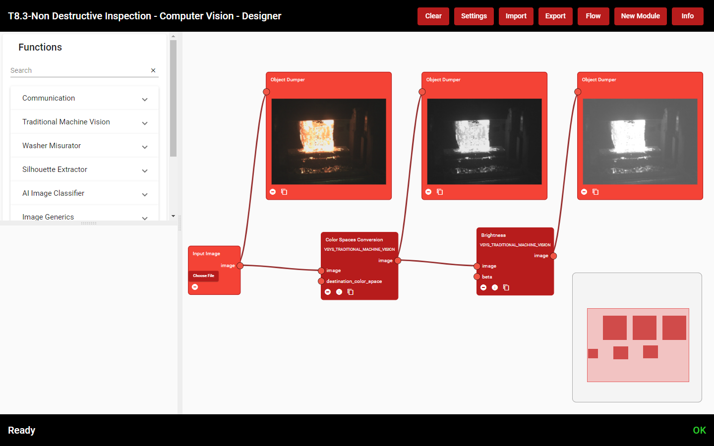
Figure 6. Use of Image Visualizer block as a debugging tool inside the Designer
The Designer can export the developed algorithm, so that the Runtime, the engine that executes algorithms, will be able to run it at run-time, for example with in-line data from cameras. The results of the algorithm can also be published in the Service & Message Bus, to allow the integration with other ZDMP Components. Multiple algorithms can be created, for multiple products, cameras, and production lines.
The component is fully modular:
A module is a package that contains a list of functions
A module should run specific algorithms and have custom dependencies
Modules and their functions are shown in the Designer
There are many Computer Vision algorithms, and a specific use case most probably will not need all of them. That is why there is a “Builder” that lets the developer choose which modules to enable. This is required when the component is run on edge PCs or embedded devices with limited hardware performance. Developers can buy modules in the Marketplace, and then they will be available for selection in the Builder. Custom modules can also be developed and uploaded when specific and new functionalities are needed.
AI Image Classification
The AI Image Classification is a tool which is part of the Non-Destructive Inspection suite. The goal of this AI-based service is the correct classification of images into different “classes”. An image can be tagged with a class, with classes arbitrarily defined by the user. The simplest case is a binary classification, where only two classes are present (for ex. good vs bad). Multi-labels scenarios are however common.
Once all the images are tagged, a training of an AI model can be executed. During this process, a Neural Network will learn to classify images from the labelled dataset (training), with the goal of reproducing this behaviour with untagged, live images (inferencing).
The inference can be executed in the Runtime component explained later.
Dataset Organization
The tool allows the user to upload and manage multiple sets of images, separated in datasets, and multiple structures, which contain the separation in classes of the images of a dataset. Each dataset can have multiple structures, which allows the user to use the same images for different classification tasks.
From the page “Upload from Local” the user can upload images to create new datasets or extend and replace existing ones, as well as uploading a pre-existing structure linked to the dataset.
Referencing Figure 7, to upload a new dataset:
“Mode” must be set to “upload”
“Name” field must not be blank
“Structure” is optional
“Upload Images” must contain at least one image
To replace a dataset: “Mode” must be set to “replace” and the id of the dataset to replace must be selected
“The user can then select “Save Dataset” to save the dataset, “Save and Load” to save and load the dataset, “Clear Cache” to clear the uploaded images / structure to start anew.
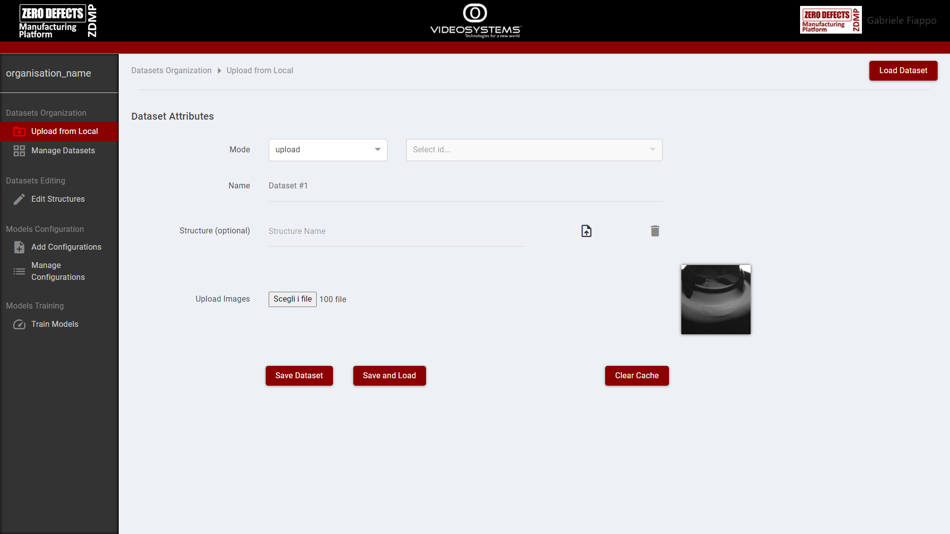
Figure 7. AI Image Classification: Upload from Local
From the page “Manage Datasets” the user can edit, expand, or delete existing datasets, as well as add or delete structures.
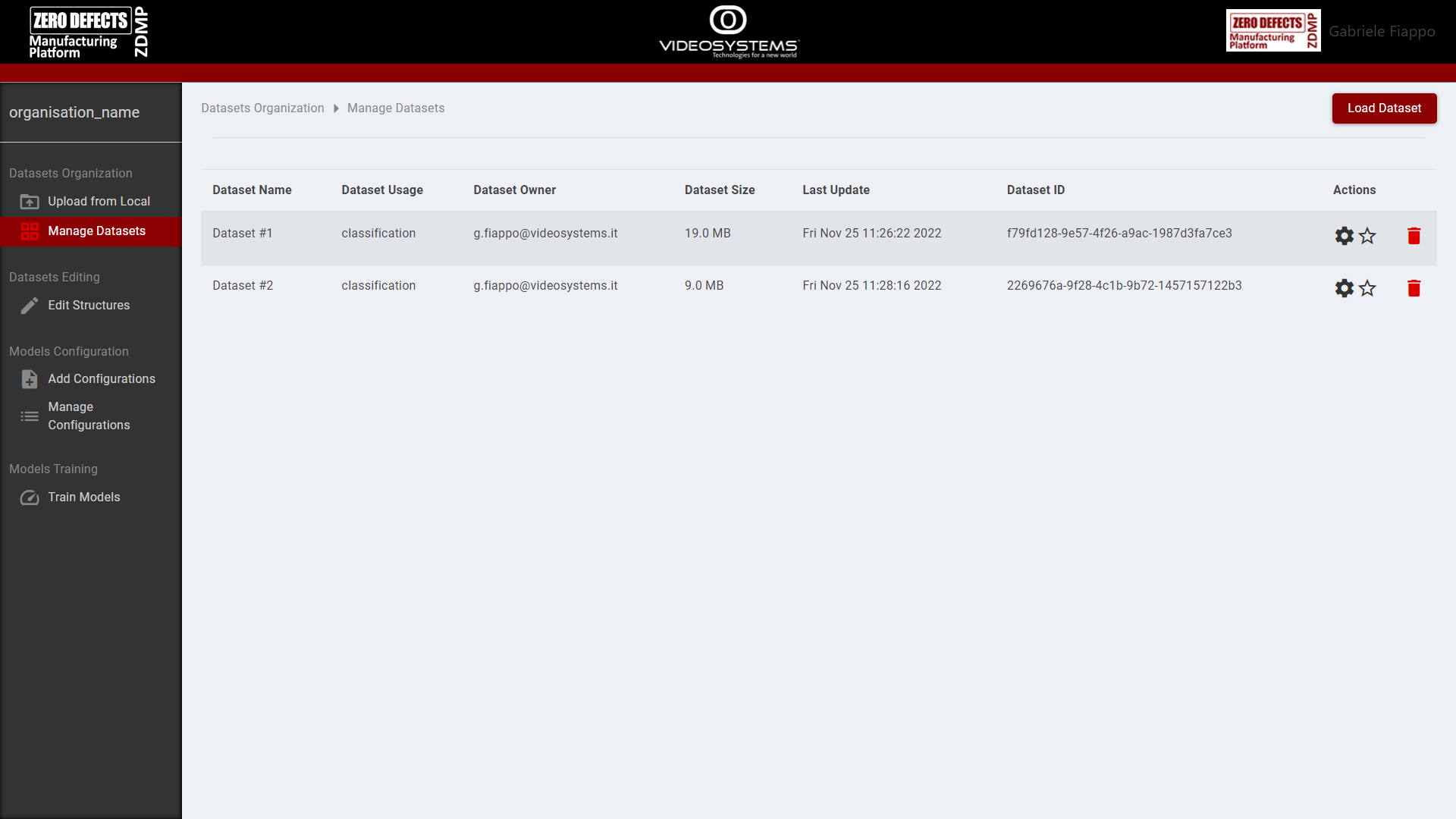
Figure 8. AI Image Classification: Manage Datasets
Dataset Editing
From the “Edit Structures” page, the user can edit structures, create classes, and move the images of the dataset between them. If no structure is already available, the tool will generate a new “standard” structure where all the images are unclassified.
Referencing Figure 9, the steps to edit a structure are:
Select a dataset with the “Load Dataset” button on the top right
Select a structure from the dropdown menu next to the “Load Dataset” button
Add a new class using the “Add Class” button
Open the unclassified class, or any class from which move / copy the images, pressing the “Set Active” button
Select the images and move / copy them to another class by hovering over the class circle and selecting “Copy here” or “Move here”
Save a new structure or overwrite the existing one using the “save” button icon next to the dropdown menu
Download the structure by clicking the “download” button icon next to the “save” button icon
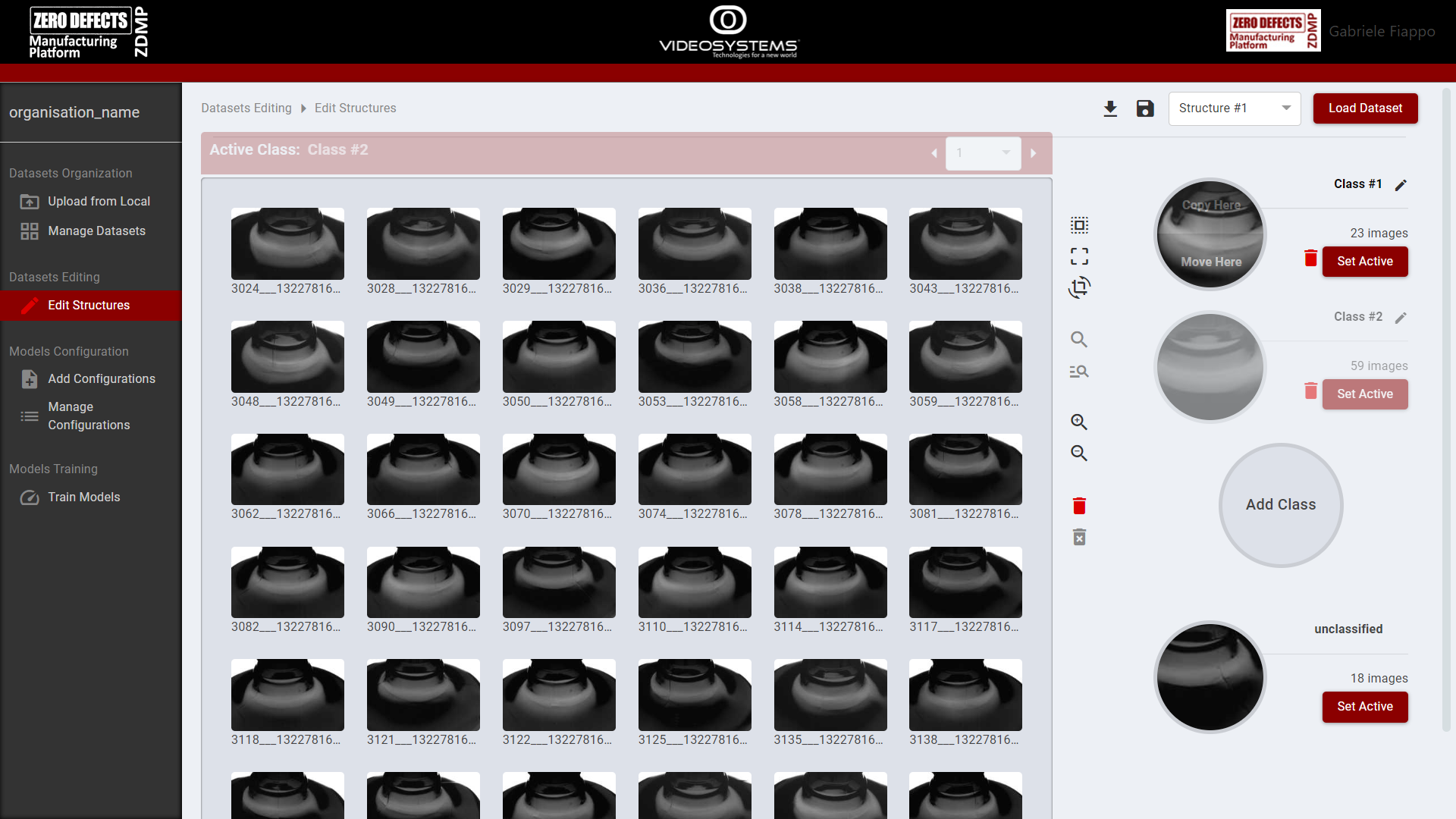
Figure 9. AI Image Classification: Edit Structures
Models Configuration
In the “Add Configuration” page, the user can select a model and set its parameters to generate a new model configuration. The available models are AlexNet and ResNet, two widely known CNN, as well as a very small TestNet useful to test parameters without having to wait long training phases.
The available parameters allow the user to configure the behaviour of standard neural network tools, like the criterion or loss function and the optimizer, as well as the parameters of the datasets and the number of training iterations.
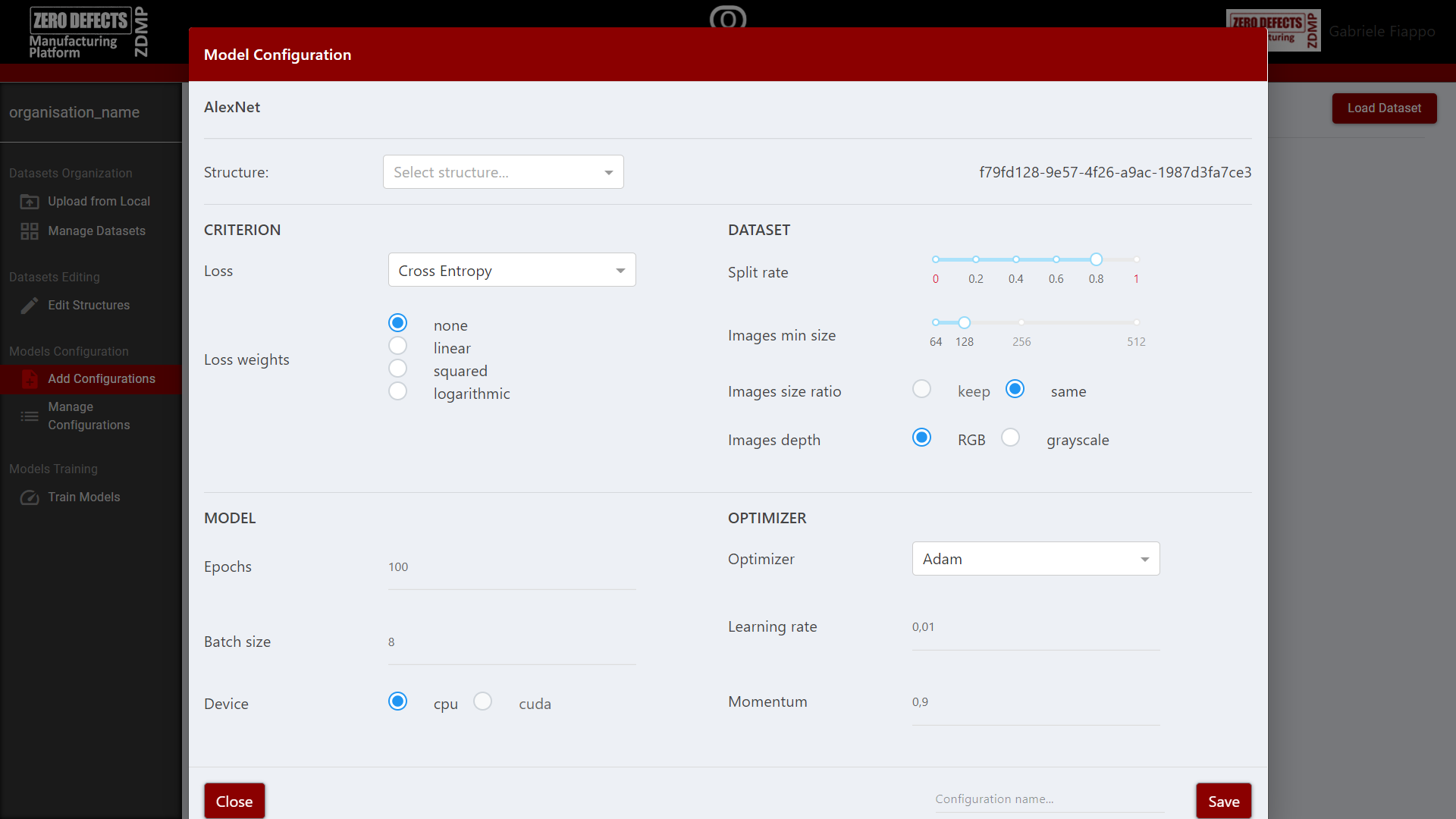
Figure 10: AI Image Classification: Model Configuration
In the “Manage Configurations” page, the user can delete a model.
Models Training
In the “Train Models” page, the user can train the model on the selected structure.
The training epochs are divided in 10 steps, shown by red squares that become green once the step is completed. Clicking on a square will show the model performance with respect to that step. The best step has a turquoise colour instead of a green one.
Once the training is completed, the user can download both the last and best versions of the model with the icon buttons near the steps.
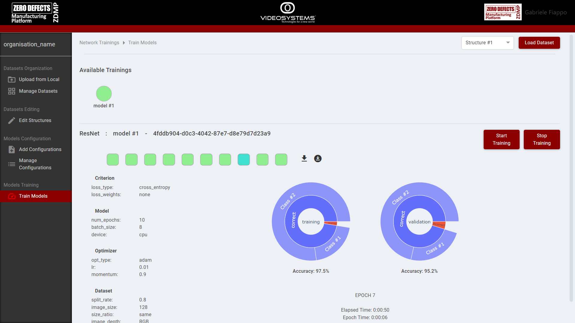
Figure 11: AI Image Classification: Train Models
Models Inference
The trained model is used to classify new images through the Runtime component. A related AI Inference module is present in the Designer (see Figure 12 and Figure 13) and its main functions foresee a model parameter to input the trained model (Figure 14).
Figure 12. AI Image Classification: Module
Figure 13. AI Image Classification: Module Information
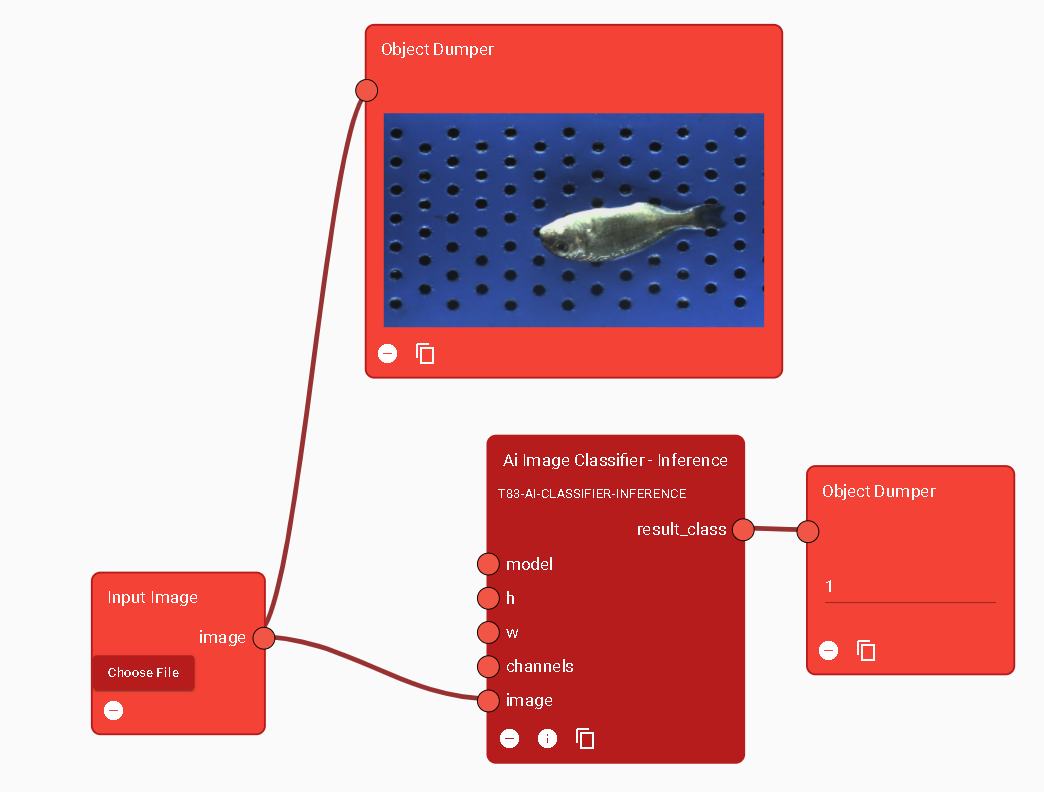
Figure 14. AI Image Inference Module: Classification Inference Function used in the Designer
AI Image Labeller
The AI Image Labeller is also tool which is part of the Non-Destructive Inspection suite. The goal of this tool is to create datasets and train neural networks to solve object detection tasks.
The AI Image Labeller allows the user to create projects, upload images, generate multiple structure that contains different classes and annotations, as well as annotate the images directly using the annotation tool and train neural networks using the trainer tool, with the goal of reproducing this behaviour with untagged, live images (inferencing).
The inference can be executed in the Runtime component explained above.
Home and Projects management
From this page, the user can create new projects from scratch. A project is the macrostructure that contains a dataset, multiple annotations and annotations’ containers, experiments, and trained model.
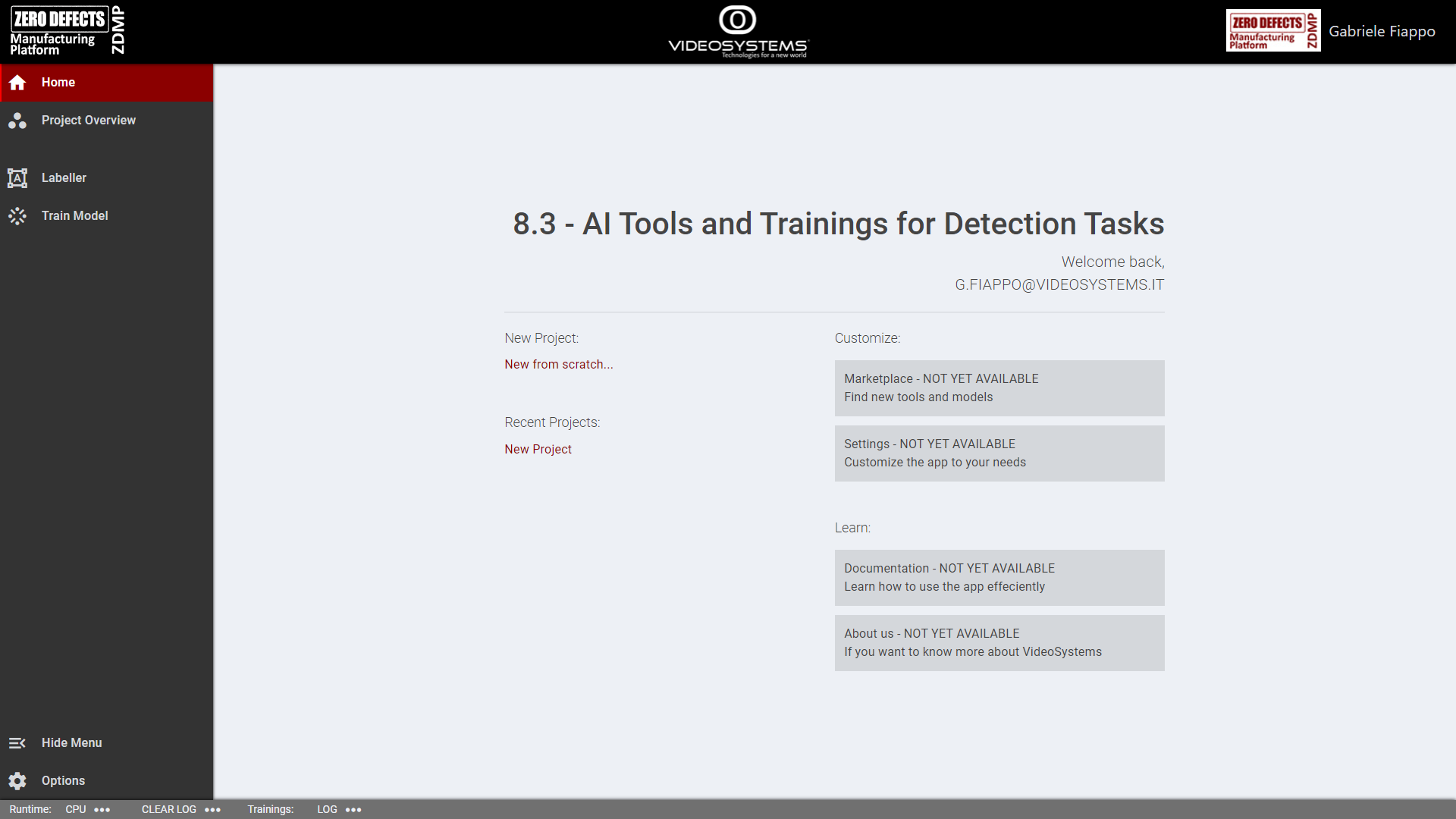
Figure 15: AI Image Labeller: Home page
Project Overview
This page contains an overview of the current projects, with available datasets and structures.
To proceed from there, the user should:
Edit the project name
Delete the current project
Upload and download images, using the icon buttons in the navigation bar
Upload pre-existing structures, using the second upload icon button in the navigation bar
Create new structures, using the “plus” icon button near the “STRUCTURES” label on the left, and select said structures
Edit the images linked to the structure, using the “collection” icon button below the structure information (the second icon button from left)
Open or delete the selected structure
Opening a structure will open the labeller interface, from where the user can annotate the images belonging to the structure.
Multiple structure can share the same images. The dataset, which contains all the images of the project, gets updated to new versions each time the user upload new images.

Figure 16: AI Image Labeller: Project Overview
Labeller
The labeller page shows the main tool of the service, the Image Labeller tool. By using this tool, the user can create classes, draw, and delete labels, change the structure name, and download the structure.
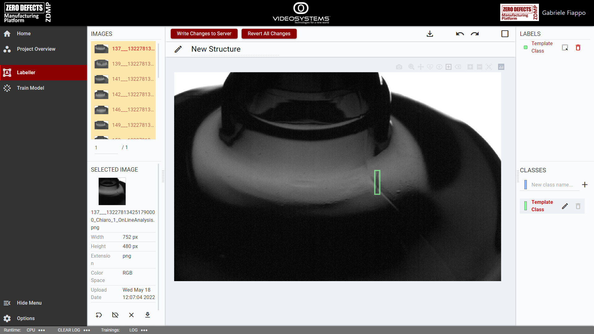
Figure 17: AI Image Labeller: page overview
The left side of the page shows a list with the available images. After selecting an image, it will be shown on the centre of the page, from where the user will be able to annotate it. Labelled images show up in yellow.
On the bottom right side, the classes are shown. A newly created structure starts with a template class, whose colour and name can be edited by pressing the icon button on its right. Each structure must always have at least one class.
Above the classes are the labels. Hovering over a label will highlight it on the image, and from the same list the labels can be deleted or converted. The conversion generates a polyline from a non-polyline label or add points to a polyline label.
Using the icon buttons on the top bar, the user can download a structure, redo, or undo a modification, and mark the image as “done”. A marked image will show up in green on the images list; this is useful to keep track of images which do not have any object to label.
After completing a labelling session, to save the modification done, the user must click the “Write Changes to Server” button on the top left of the labeller. Failing to do so will cause the loss of the newly done labels.
The “Revert All Changes” button will revert all changes done during the session instead.
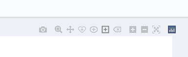
Figure 18: AI Image Labeller: labeller button bar
The labeller button bar shows all the tools available. From left to right, the available tools are:
Snapshot: to download the image
Zoom: to zoom the image on a given area
Move: to move the image around
Close freehand: to create close polygonal annotations with freehand drawing
Circle: to create circle and ellipse annotations
Rectangle: to create rectangular annotations
Erase: to delete a selected annotation
Zoom in
Zoom out
Autoscale: to bring the image back to the original scale
Train Model
This page allows the user to create new experiments (trials) to train neural networks on a specific structure.
After having select a model on the left, the user can edit various parameters:
The first tab (training) contains the more generic parameters, such as the number of epochs, which structure to use, the images and batch size
The second tab (Model) shows the parameters specific to the model
The third tab (optimizer) let the user show an optimizer and its parameters
Before starting the training, the user must name the trial. The name must differ from the name of other trials already available.
Completed these steps, the user can start a training by clicking on the “Start” icon button. The training will start, and progress will be shown both in the log on the right and in the charts below the trial configuration.
After the training is done, the user can download both the last and the best epochs, using the icon buttons near the “Start” icon button.
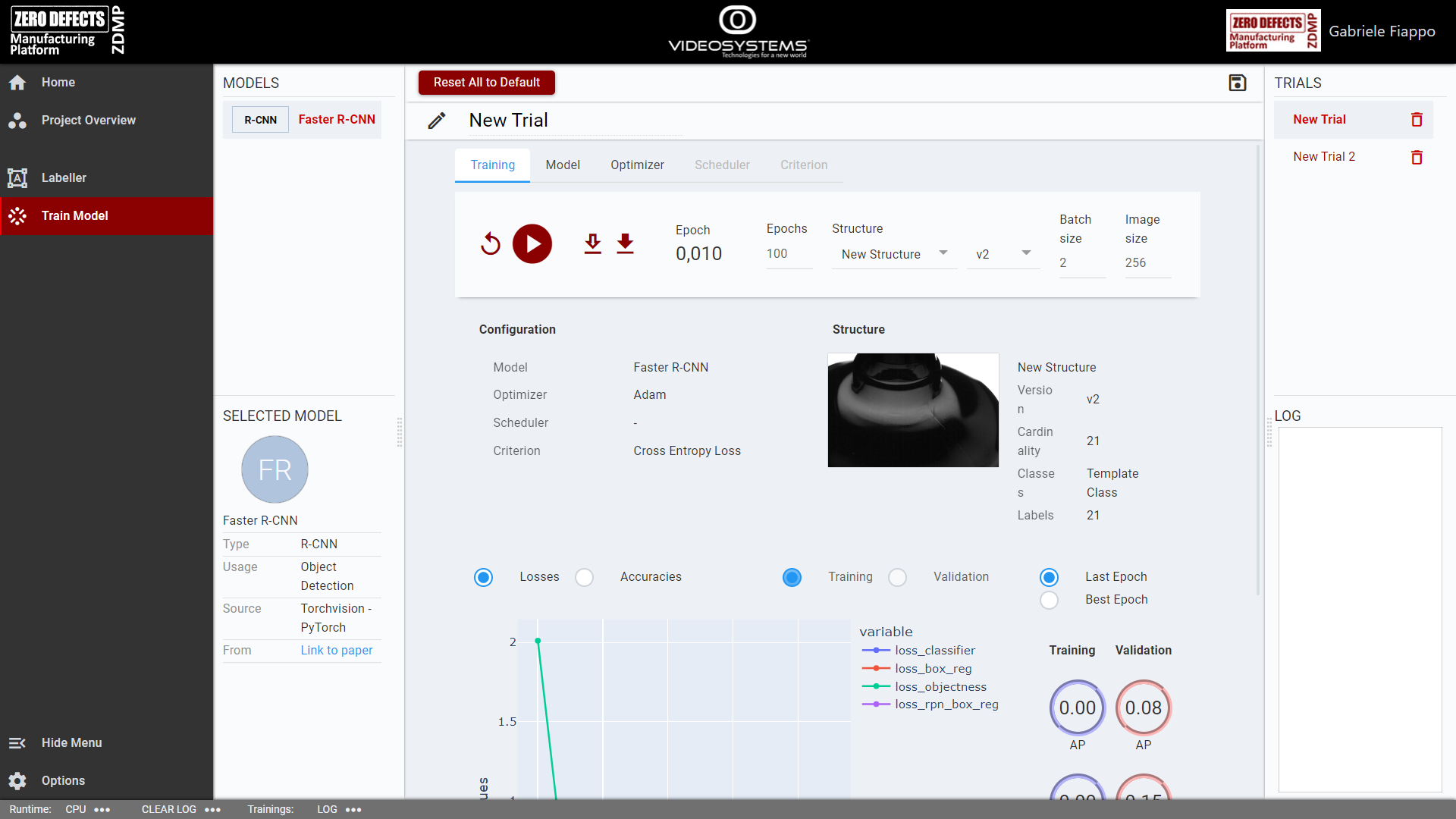
Figure 19: AI Image Labeller: Train Model
System Requirements
The component is managed by the Application Runtime. All the component’s software requirements are automatically resolved.
As the component is very flexible and can be used to run a multitude of algorithms, hardware requirements may vary depending on the frequency of process requests, the size of files and images, and the techniques used. Some modules, based on Machine Learning and Neural Networks, may require one or more GPUs if the process time is a crucial factor.
In general, developers should run some tests to judge how many resources are needed. The component will auto-scale as needed to use all the available resources. If the component requests resources which are not available, it is necessary to upgrade the hardware.
This is an edge component, which means it can be installed in the edge layer.
| Software |
|---|
| Application Runtime |
| Hardware |
| 8+ CPUs |
| 16GB+ RAM |
| 100GB+ disk |
| x nVIDIA CUDA Capable GPUs (if any module needs them) |
Associated ZDMP services
Required
Secure Authentication and Authorisation: This is needed to secure the communication between components and authorize API calls
Portal: Needed to access all services within the platform, centralizing the authentication procedure
Marketplace: The modules created by developers must be uploaded to the Marketplace. Users can then buy modules based on their needs and those modules will be available in the Builder component
Service and Message Bus: The component is needed for the communication between the Runtime component and a zApp or another component
Application Runtime: Needed to build and run the component and any EXTERNAL_IMAGE modules
Optional
Data Acquisition: The Data Acquisition component exposes images from cameras inside the platform to be analysed
Storage: The Storage component stores images for later processing
Installation
Once bought in the Marketplace, the component is available for installation through the Secure Installation component. Some installation variables can be set:
“Private Registry Settings”
“Private Registry URL”: the ZDMP container registry URL
“Private registry user/password”: the login for the ZDMP container registry.
“Builder Backend - Authentication”
“The realm this instance is referenced to”
“Human Collaboration Registry URL”: the ZDMP Human Collaboration container registry URL
“Human Collaboration Registry user/password”: the login for the ZDMP Human Collaboration container registry
“Builder Backend - Ingress”
“Enable Ingress”: enable Ingress
“Ingress Host”: URL of the Builder Backend component
“Ingress Path”: leave default
“Builder UI - URIs”
“Public URL of the Designer”
“Public URL of the Component”: leave default
“Public URL of the Builder Backend Component”: URL of the Builder Backend Component, the same as the one in the “Builder Backend - Ingress”
“Public URL of the Portal Component”
“Builder UI - Ingress”
“Enable Ingress”: enable Ingress
“Ingress Host”: URL of the Builder UI component
“Ingress Path”: leave default
“Runtime Designer - URIs”
“Public URL of the Builder”
“Public URL of the Component”: leave default
“Public URL of the Runtime Backend Component”: URL of the Runtime Backend Component, the same as the one in the “Runtime Backend - Ingress”
“Public URL of the Portal Component”
“Runtime Designer - Ingress”
“Enable Ingress”: enable Ingress
“Ingress Host”: URL of the Runtime Designer component
“Ingress Path”: leave default
“Runtime Backend - Ingress”
“Enable Ingress”: enable Ingress
“Ingress Host”: URL of the Runtime Backend component
“Ingress Path”: leave default
“Deployment Options”
“Deploy on the same Node (if possible)”: replicas of the component are instantiated on the same node, to improve performance. Ignore this if installing on a single-node cluster
“Force deploy on the same Node”: force instantiation of the replicas on the same node
“Persistence”
“The Filesystem Storage size”: size of the Filesystem Storage
“The Internal Filesystem size”: size of the Internal Filesystem
“AccessMode”: leave default
“Volume Type”: nfs or local
“StorageClassName”: leave default
“PersistentVolumeReclaimPolicy”: leave default
“HostPath for same node installations”: if “Volume Type” is local, this indicates the path on the node to the Volume
“NFS Server URL”: if “Volume Type” is nfs, this is the URL to the NFS Server
“NFSPath for multiple nodes installations”: if “Volume Type” is nfs, this is the path where to setup the Volume.
How to use
The Component is divided in three parts:
Building phase
Designing phase
Runtime phase
In the Building phase, the Developer chooses which modules to enable in the Designer and Runtime Component. Additional modules must have been previously purchased through the Marketplace to be available in the Builder UI. The Developer, via the Builder UI, will choose which modules are needed for the specific algorithm to be built.
In the Designing phase, the Developer will use the enabled modules by graphically building an algorithm connecting modules’ functions via the UI.
In the Runtime phase, real-time or historic images can be processed through the developed algorithm.
Builder
The Builder allows selection of which modules to include in the Runtime Component. The modules can be purchased through the Marketplace and can be enabled here. Once the building procedure is done, the selected modules will be available in the Designer and the Runtime Component for run-time processing.
The image of Figure 20 shows the Builder UI where three modules are present. The Learn More button gives more detailed information on a module. Check a module version to make it available inside the Runtime Component. Multiple versions of the same module can be checked, in which case the versions will coexist. This is useful, for example, to test the latest version of a module without removing the old version which is running in production. In this example, the Traditional Machine Vision and the PyTorch Inference modules are selected, ready to be built.
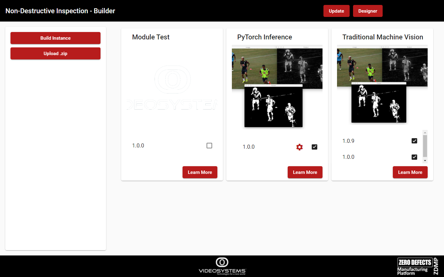
Figure 20. The Builder UI
The Build Instance button is used to build Runtime Component. Subsequently, the Runtime Component will be ready, and the Designer, which will be described just below, will be accessible from the Designer button.
Designer
The Designer allows a developer to visually build Computer Vision algorithms.
This tool facilitates the development of an algorithm. The user can build a complex and specific flow using graphic debugging tools and the documentation of each module. It is particularly useful for pre-processing purposes, also considering that there is an infinite number of cameras and sensors in the market, with various characteristics, and the environmental conditions are a particularly key factor. This tool allows an algorithm to be tested with different images from different cameras and this way it is easy to check if the algorithm is stable or it needs to be tweaked, as necessary.
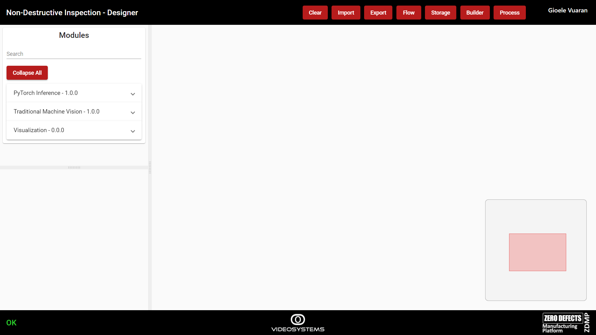
Figure 21. The Designer
On the left side, the list of the built modules is shown and for each of them the menu can be expanded to show their functions as well. To add a Function to the flow, click on Add, and the function block will be inserted in the Designing canvas.
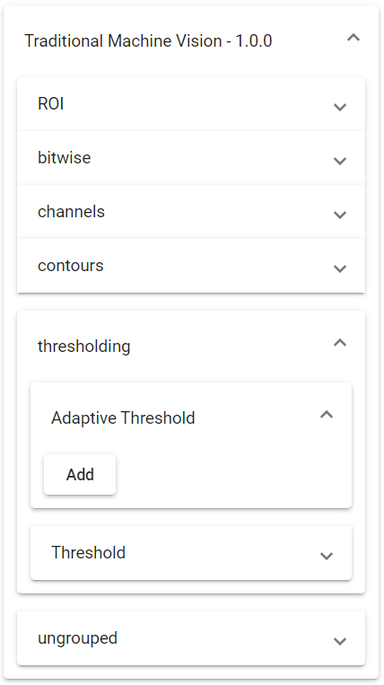
Figure 22. The Functions of the Module Traditional Machine Vision
Every Function has input and output parameters. An output parameter of a Function can be connected to an input parameter of another one. Every parameter has a type: only parameters that have the same type can be connected; for example, an Image parameter cannot be connected to an Integer one.
In the image of Figure 23, the output parameter “image” of the Function Colour Spaces Conversion is of type IMAGE, and it is connected to the parameter “image” of the Function Threshold, which is of type IMAGE too.
At the bottom of each Function block at least three Ease-of-Use icons are displayed; from left to right they allow respectively to: remove the Function block, open an information window describing the Function, and duplicate the Function block in case more than one is needed to construct the algorithm in the Designer canvas.
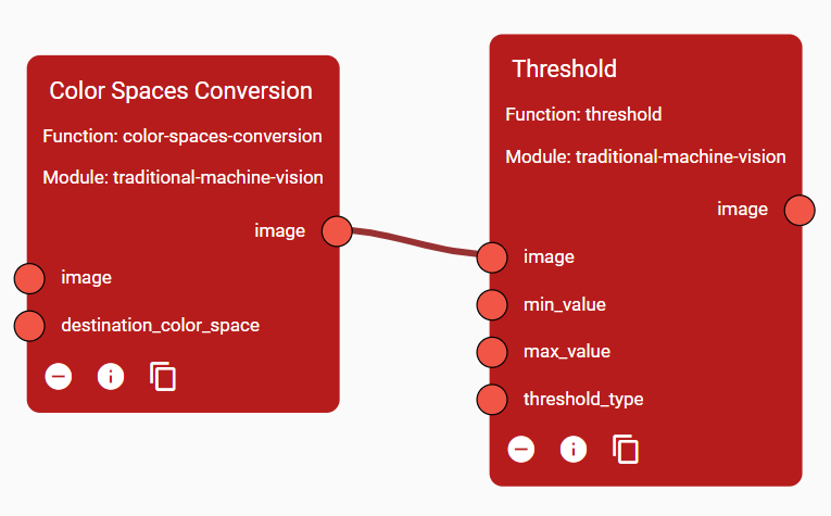
Figure 23. Two Functions connected
This is a basic step to create an algorithm. Obviously, through multiple steps and/or more sophisticated functions, the complexity of the algorithm is increased: this is often the case in Machine Vision analysis to address specific applications.
Once an algorithm has been completed, and usually tested, it can be exported by clicking on the Export button. This will download a .json file containing a recipe. The recipe contains all the logic needed from the Runtime to process data at run-time. Multiple recipes can be created, for various products, cameras, algorithms, etc. These files should be stored by the ZDMP Developer to later be used at run-time when needed.
There are several functions used to debug a specific algorithm. For example, the “Input Image” Function is used to load an Image from a user PC to test the algorithm. The “Object Dumper” prints the connected parameter’s value. In the image of Figure 24 some debugging functions have been added to the flow and an image has been uploaded from the PC to test the algorithm. What each Function is doing becomes clear.
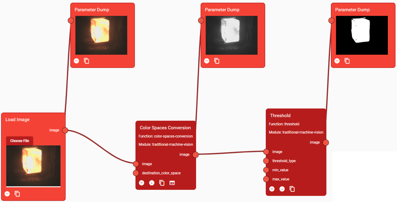
Figure 24. A simple algorithm with some debugging blocks to monitor processing step by step
The input parameters of a Function can be edited. When a Function is selected with a left click, a menu will appear on the left side. This allows the user to change the Selected Function’s Parameters.
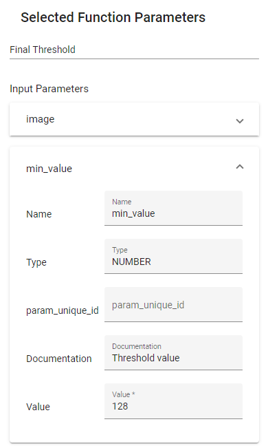
Figure 25. Selected Function Parameters
Figure 25 shows an example of Selected Function Parameters. At the top, the Function’s display name can be edited. It is then possible to see the list of input parameters of the selected Function. Click on each parameter to edit its value. The type of the parameter is also shown. Different input methods are available depending on the type of the parameter. If a parameter is connected to another Function’s output, changing its value is not possible as it would not make sense.
The values of parameters set here are embodied in the algorithm exported via the Export button. When a process is executed, the Runtime will, by default, take the values from the exported algorithm, so they are hardcoded. The param_unique_id property is used to flag a parameter to make it overridable at run-time when a process is executed. Each parameter to be exported for this purpose must have a unique param_unique_id.
For example, in the flow of Figure 24 it makes sense that the input image of the first function block is to be overwritten with new images from a camera. This is not limited to images: the min_value parameter of the Threshold Function can, for example, depend on a light sensor: if the light sensor reports a very bright environment, the threshold value can be lowered, and vice versa.
In the example of Figure 26, the parameter image of the first Function in the flow, Colour Spaces Conversion, has been flagged “input_image”.
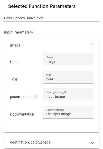
Figure 26. The param_unique_id flag of an input parameter
A similar thing can be envoked for the output parameters. By default, output parameters of functions are not returned as results, because that would impact the performance and most of them are of minor interest for the final application. Again, only if the param_unique_id property is set, that parameter will be returned. In the example above, the result of the algorithm, which is the output parameter image of the Function Threshold, can be flagged as in Figure 27, so that at run-time the user will receive it within the results.
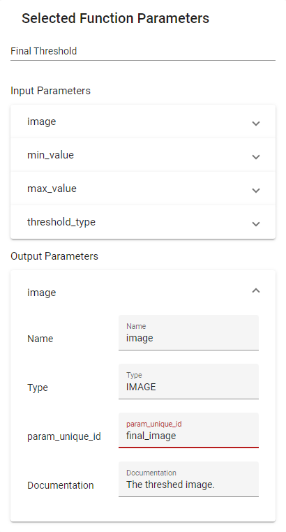
Figure 27. The param_unique_id flag of an output parameter
Some functions can also have a UI, which can be used to simplify the editing of the input parameters. Henceforth, it will be referred as Function UI. If a module’s function has a Function UI, an additional far-right icon will appear at the bottom of the function block as in Figure 28. Clicking on it will open a dialog.
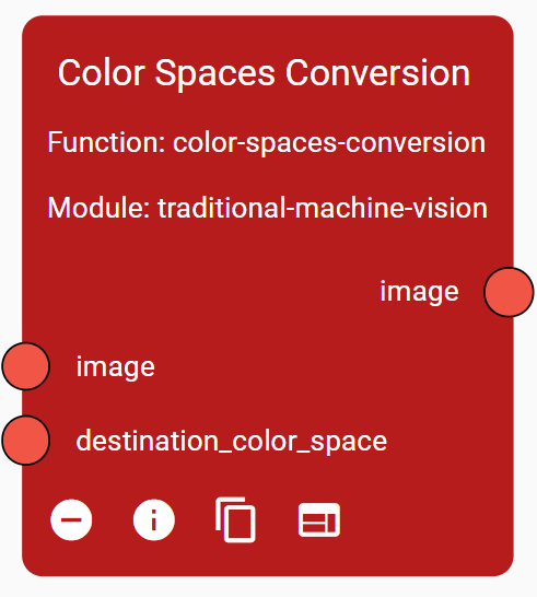
Figure 28. A Function with a Function UI
The image of Figure 29 shows an example of a Function UI. In this example, the input parameter “roi” is edited graphically.
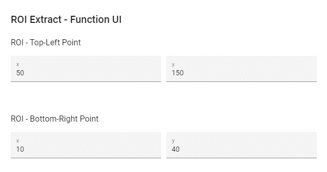
Figure 29. A Function UI
This can also be achieved by directly editing the Function Parameters, as shown in Figure 30, although the Function UI may help if the parameter is complicated.
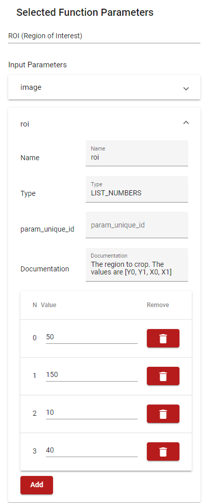
Figure 30. Updating an input parameter from the Selected Function Parameters menu
Runtime
The Runtime is the API Server of the Component. It runs algorithms at run-time. The Runtime REST APIs are accessible via API Gateway of the Service & Message Bus component.
The OpenAPI specification file to communicate with the component can be found in the API Gateway or it can be accessed in the technical documentation of the project at https://software.zdmp.eu/docs/openapi/edge-tier/non-destructive-inspection/openapi.yaml/. For more info on OpenAPI, https://swagger.io/docs/specification/about/.
The Runtime is used to execute a processing based on recipes exported from the Designer. The following APIs expose functions to allow this:
Set Flow Recipe (/flow/set)
Run Flow Recipe (/flow/run)
Flow API – Set Flow Recipe
Recipes must be uploaded to the Runtime before executing a Run Flow command. The Set Flow Recipe API requires:
Filename: The filename of the recipe file, for example check_dimensions.json
Body: The recipe to be set
This will save the recipe in the internal storage with the provided filename. This way recipes can be set only once. Figure 31 shows the Designer’s Storage dialog with the recipe file.
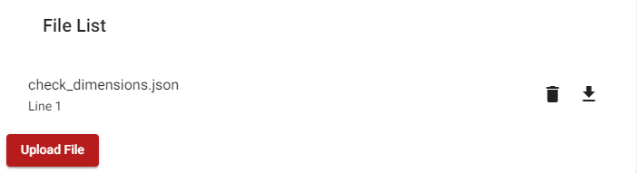
Figure 31. The recipe file is saved in the Internal Storage
Flow API – Run Flow Recipe
To run a processing on some data, the Run Flow Recipe API must be called. This requires:
Filename: The filename of the recipe previously uploaded
Input Params: List of input parameters (please check the param_unique_id above)
ID: String that will be sent back in the response, useful for tracking the inspected product or the processing analysis
It returns:
Output Params: List of output parameters (please check the param_unique_id above)
Flow Response Times: Object containing how much time each function and the whole algorithm took, useful for debugging purposes
ID: The same ID passed in the request
The following diagram shows an example of how to use the Runtime APIs; the following steps are taken:
Setting up the “check_dimensions” recipe
Setting up the “check_cracks” recipe
Running a Flow process using “check_dimensions” recipe
Running a Flow process using “check_cracks” recipe
Running a Flow process using “check_cracks” recipe
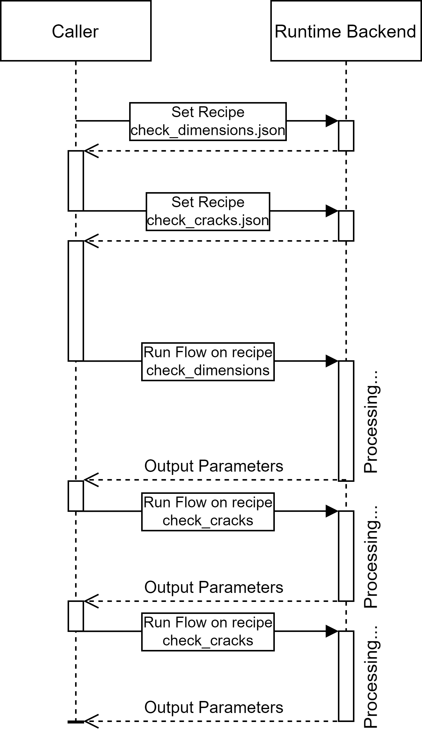
Figure 32. Demo of SetFlow and RunFlow
Internal Filesystem Storage
The component is equipped with an internal filesystem storage. It is used to store images, files, and data, so they can be used inside an algorithm.
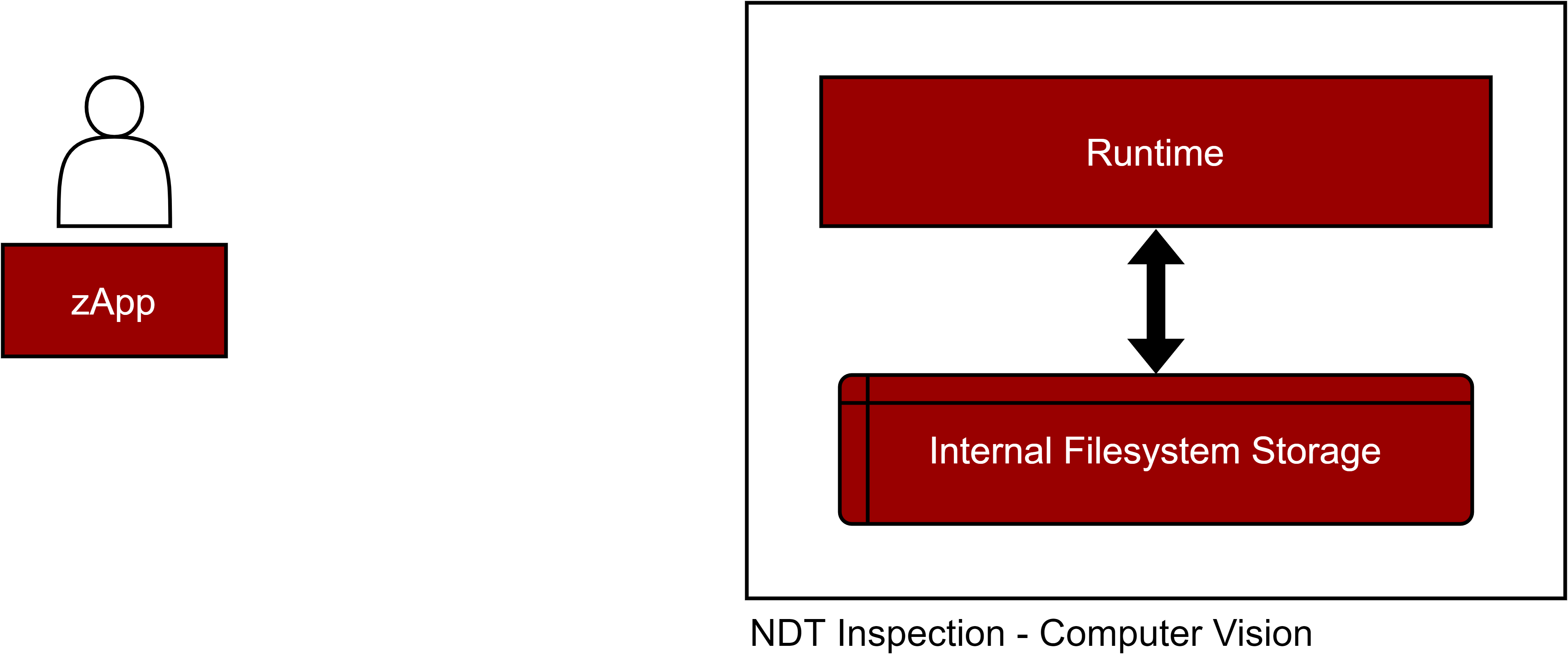
Figure 33. NDT Inspection - Computer Vision component schema
There are three ways to interact with the Internal Filesystem Storage:
- Designer
Files can be uploaded from the Designer by clicking on the Storage button.
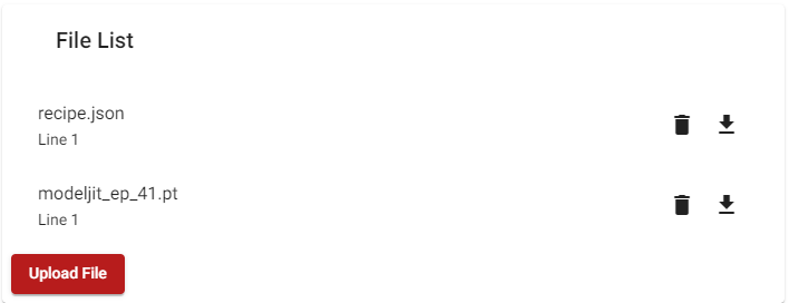
Figure 34. Designer: Upload files to the internal storage
Runtime APIs
- Runtime APIs
Files can also be uploaded via HTTP API (please check the OpenAPI specification):
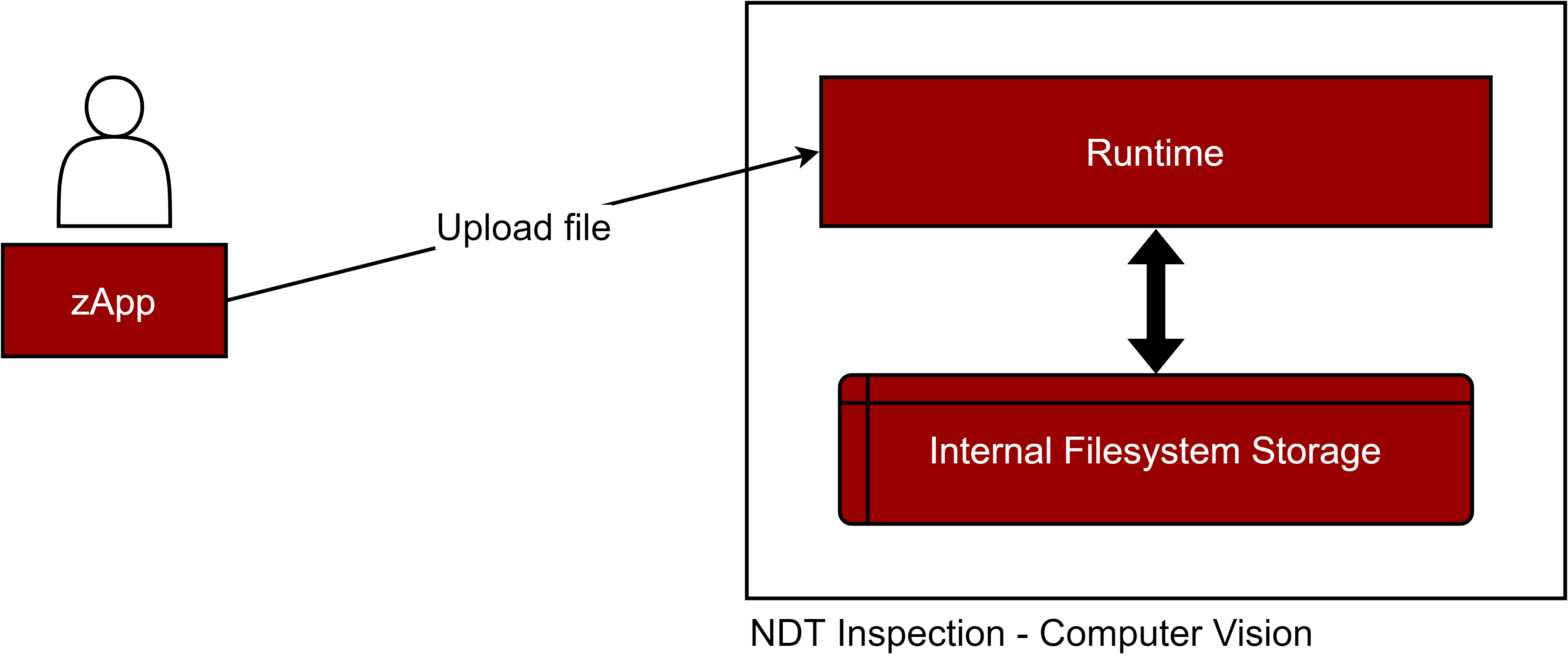
Figure 35. CRUD files via REST APIs
- Persistent Volumes
The Internal Filesystems Storage can also be mounted as a Persistent Volume. While this is the fastest way to read and write files, it requires additional configuration from the Application Runtime component. This solution is preferred in low latency-edge scenarios.

Figure 36. CRUD files by mounting the Volume
Parameter Model Description
The request and response object of the Run Flow Recipe API contain, respectively, a list of input and output parameters. Here the Parameter model is described.
| Field | Mandatory | Type | Description |
|---|---|---|---|
| name | true | string | The name of the parameter |
| value | true | any | The value of the parameter |
| type | true | enum | The type of the parameter. [ ALL, NONE, NUMBER, LIST_NUMBERS, STRING, LIST_STRINGS, BOOLEAN, IMAGE, LIST_IMAGES, FILE, LIST_FILES, OBJECT] |
| min | false | float | The minimum value allowed for the parameter. Used for NUMBER types |
| max | false | float | The maximum value allowed for the parameter. Used for NUMBER types |
| step | false | float | The min step value allowed for the parameter. Used for NUMBER types |
| param_unique_id | false | string | ID used to update a parameter when calling the Flow APIs or used to export a parameter in a Flow API call. Please read above |
| file_type | false | enum | The serialization method of the parameter. Used for IMAGE and FILE types. [RAW_B64, FILESYSTEM_STORAGE] |
The APIs accept application/json data, so there are no problems when providing JSON serializable values, like integers, floats, strings, etc. Images and files, however, require serialization to be sent via HTTP. The file_type field is used to indicate how images and files are serialized. It can be set to:
RAW_B64: the image or the file is encoded to a base64 string. The value field will contain the encoded string. This is recommended when dealing with small images and files
FILESYSTEM_STORAGE: the image or the file is present in the internal filesystem. The value field will contain the filename (ex. trained_model.onnx). To save a file or image to the internal storage, please read the relative documentation above. This is recommended when dealing with large images and files
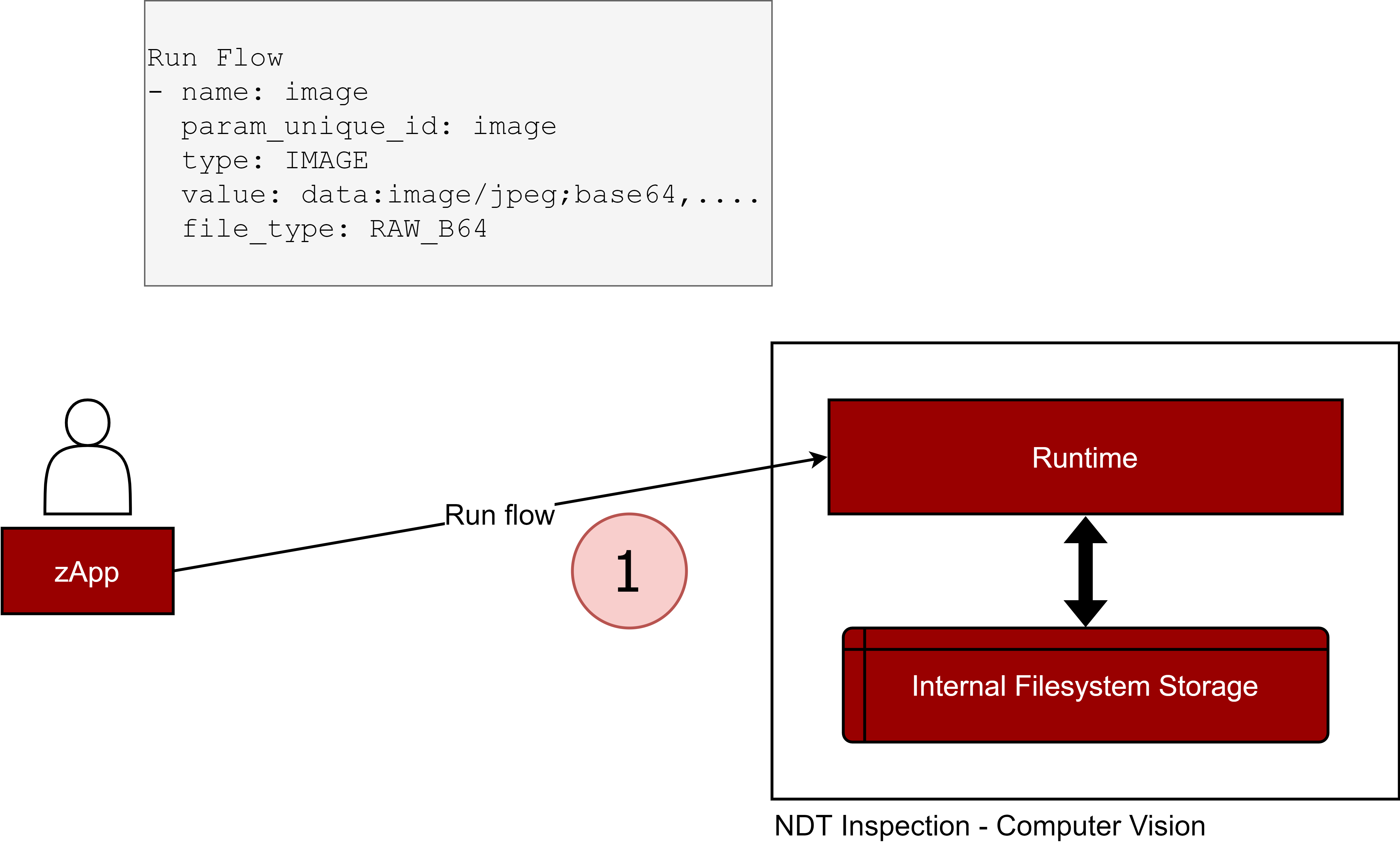
Figure 37. RunFlow with a RAW_B64 IMAGE parameter
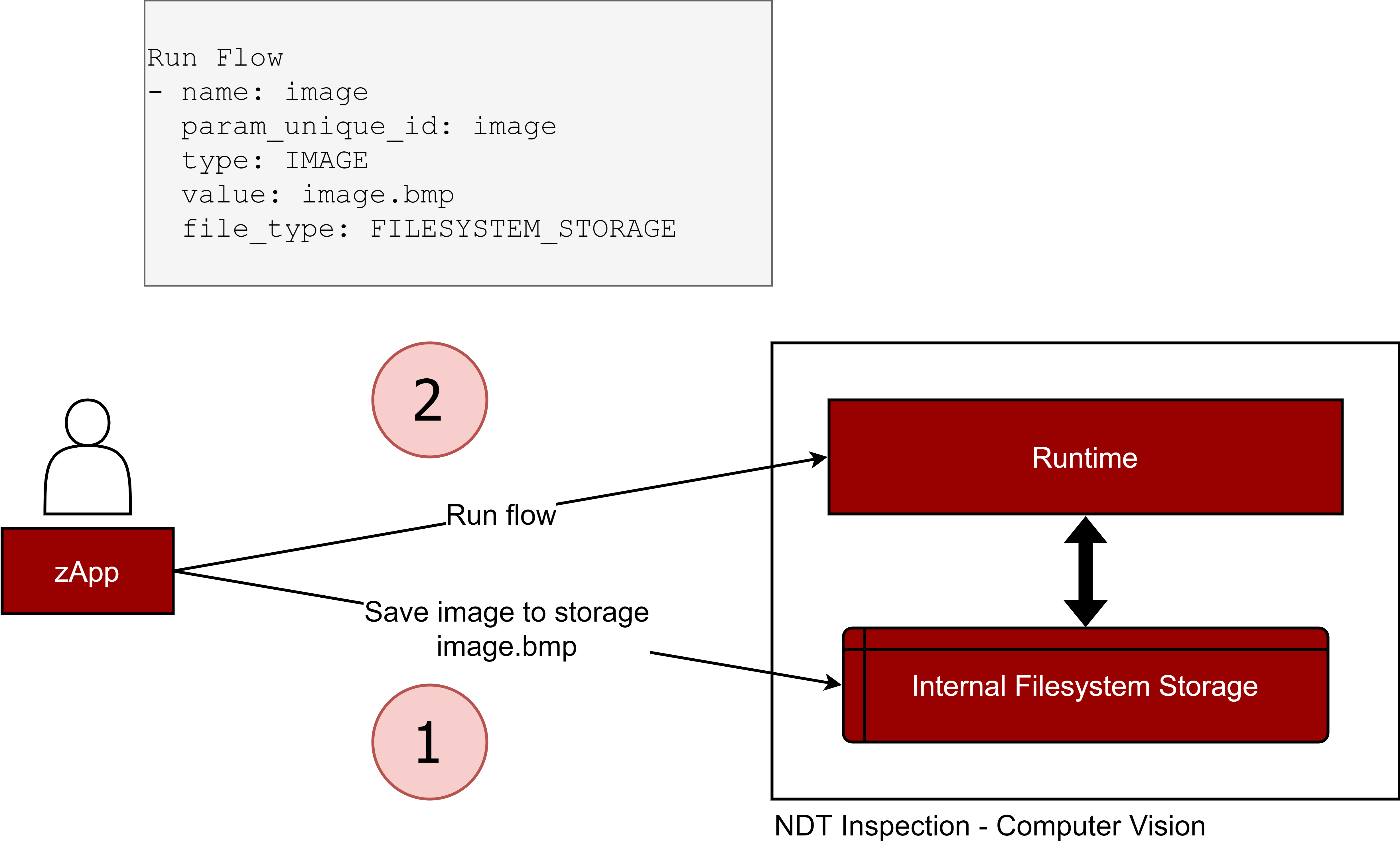
Figure 38. RunFlow with a FILESYSTEM_STORAGE IMAGE parameter
Develop a Module
A module is a package which contains a list of functions. Developers can develop their own module if a feature is missing and then use it inside the Runtime component. Some Computer Vision algorithms are extremely fast and require only a few dependencies. Neural Network based algorithms, however, are heavy and require custom dependencies, OSs, and computational resources such as GPUs. The Component gives the ability to develop new modules with distinct characteristics. That is why there are three types of modules.
DIRECT: The first one is the simplest and fastest as the functions are executed directly on the Runtime. The trade-off is the Module must be written in Python and custom libraries cannot be installed
PYTHON_EXTERNAL_IMAGE: The second one consists of a Container which runs the Python functions. In this case, custom Python libraries can be installed, and the functions will be executed in an isolated environment
EXTERNAL_IMAGE: The third one consists of a generic Container used to run more advanced functionalities. This can be written in the programming language of choice and be configured with all the needed hardware resources, so there are no constraints
There is a tool that can help with the creation of a module: the Module Creator utility. With the Module Creator utility new modules can be created from scratch or previously created modules can be edited. Functions can be immediately tested as they are being edited. This allows a fast development and debugging of modules.
For the first two types of modules, the Python source code can be edited using the built-in Python editor. For the EXTERNAL_IMAGE module, users develop their own container with their desired algorithms, but this is a higher level of complexity.
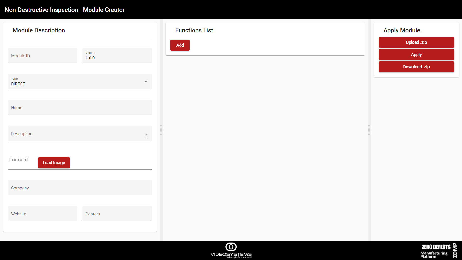
Figure 39. Module Creator page
The module must be exported by clicking on the Download .zip button, and then it must be uploaded to the Marketplace. Then, it will become available in the Builder UI.
Module Description
On the left side of the page, there is the Module Description editor, which allows editing of the new module’s basic information, such as the name, the description, etc. In particular:
| field | Meaning |
|---|---|
| Module ID | The unique ID of the module. This is the Marketplace module name |
| Version | The version of the module |
| Type | Module Type: [ “DIRECT”, “PYTHON_EXTERNAL_IMAGE “, “EXTERNAL_IMAGE”] |
| Name | Name of the module |
| Description | Description of the module |
| Thumbnail | Logo |
| Company | Developer’s Company |
| Website | Company’s Website |
| Contact | Developer’s contact e-mail |
Figure 40 shows an example of a filled-out Module Description:
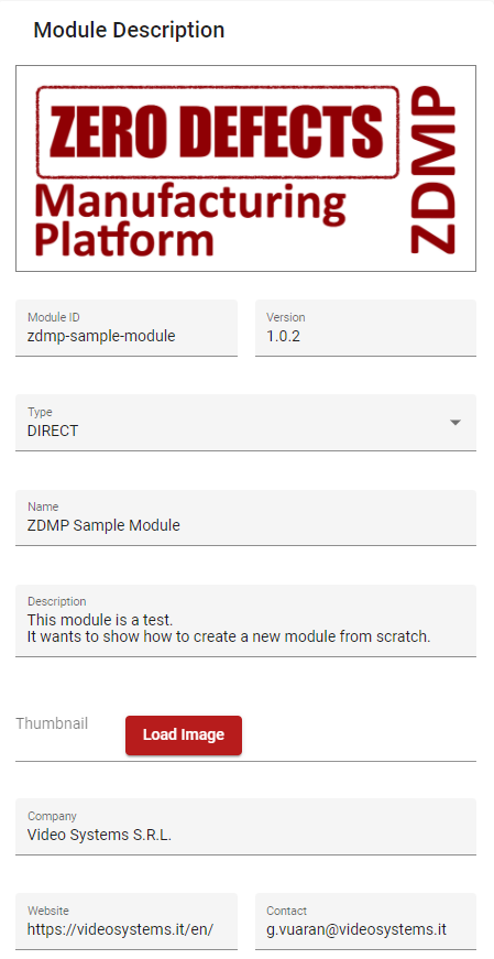
Figure 40. Module Creator - Module Description example
Functions List
On the centre of the page, there is the Functions List editor. It allows adding Functions to the module. Click on Add to add a Function. The user can expand the newly created Function by clicking on the arrow.
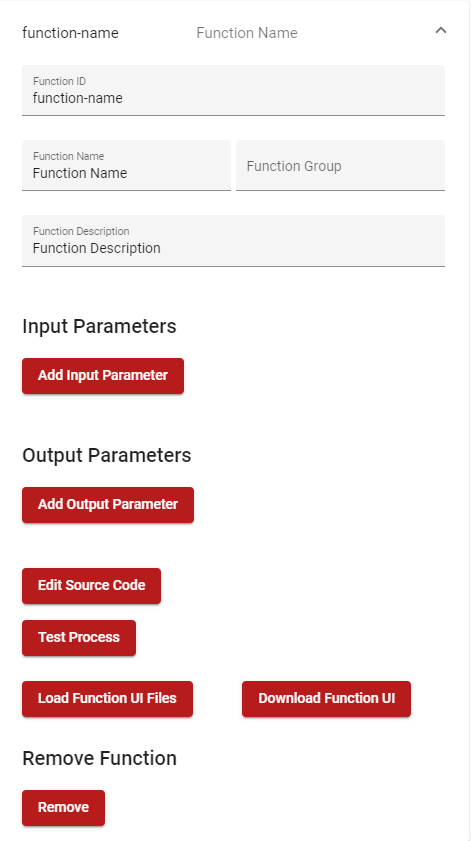
Figure 41. Module Creator - Functions List
| Field | Meaning |
|---|---|
| Function ID | The ID of the Function. It must be unique in the module |
| Function Name | The name of the Function |
| Function Group | (Optional) Graphical Function grouping |
| Function Description | Description of the Function |
| Input Parameters | Definitions of the Function’s input parameters |
| Output Parameters | Definitions of the Function’s output parameters |
| Edit Source Code | Opens the Function Code Editor Dialog |
| Test Process | Opens the Function Test Process Dialog |
| Load Function UI Files | (Optional) Upload a Web Component associated with the function |
| Download Function UI | Downloads a .zip file containing the uploaded Web Component |
To add an Input or Output Parameter, click on the corresponding button. Then the newly added Parameter can be edited, as shown in Figure 42.
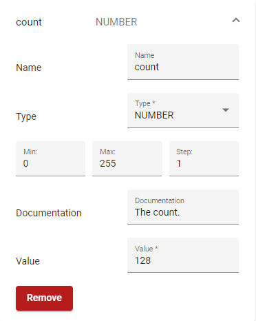
Figure 42. Module Creator – Edit Function Parameter
| Field | Meaning |
|---|---|
| Name | The name of the parameter. It must be unique in the Function’s input or output parameters |
| Select | The type of the parameter. allowed_values = [“ALL”, “NONE”, “NUMBER”, “LIST_NUMBERS”, “STRING”, “LIST_STRINGS”, “IMAGE”, “LIST_IMAGES”, “FILE”, “LIST_FILES”, “BOOLEAN”] |
| Value | The parameter’s default value |
| Step | The parameter’s step value (in case of a NUMBER type) |
| Min | The parameter’s min value (in case of a NUMBER type) |
| Max | The parameter’s max value (in case of a NUMBER type) |
| Parameter Documentation | Documentation of the parameter |
The Remove button will remove it from the list.
Function UI
Functions can also provide a UI to easily configure the input parameters. The Function UI is a Web Component (https://developer.mozilla.org/en-US/docs/Web/Web_Components). Web Components can be created from multiple frameworks (https://github.com/obetomuniz/awesome-webcomponents#libraries-and-frameworks). Angular has Angular Elements (https://angular.io/guide/elements).
The files that need to be uploaded are these two. If the framework of choice generates multiple files, they need to be concatenated:
index.js
style.css
The name of the Custom Element must be function-ui.
customElements.define('function-ui', ....);
The Web Component must also define “getter” and “setter” properties to be able to pass and retrieve data:
| Input Data | Meaning |
|---|---|
| input_params | List of Function’s input parameters |
| output_params | List of Function’s output parameters |
The Function UI should be used when a function has a lot of parameters, they are difficult to set (eg lists), or the developer wants to give the user a custom UI feedback.
For example, the function called ROI is used to crop a part of an image. It has:
A parameter called image representing the input image
Another called rectangle, of type LIST_NUMBERS, where each value is the vertex of the rectangle used for cropping
While the rectangle parameter value can be set from the Selected Function Parameters menu explained earlier, it is not an easy task. The image size must be known when setting the vertices and it requires some trial and error before finding the correct pixel values.
The Function UI can help in these situations: a Web Component can be developed which displays the input image (from the image parameter) and a rectangular selection box representing the input parameter rectangle. When the rectangle moves or is resized, the input parameter is updated accordingly.
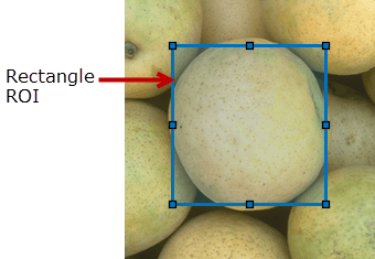
Figure 43. Function UI example
The Designer will get the input_params property of the Web Component when the user closes the dialog to update the flow.
Function Code Editor
When developing a DIRECT or PYTHON_EXTERNAL_IMAGE module, the Function Code Editor Dialog will display a built-in editor where the processing code can be edited. The buttons on the right:
Set Code confirms the changes made to the code
Reset Code clears the code and pastes a template
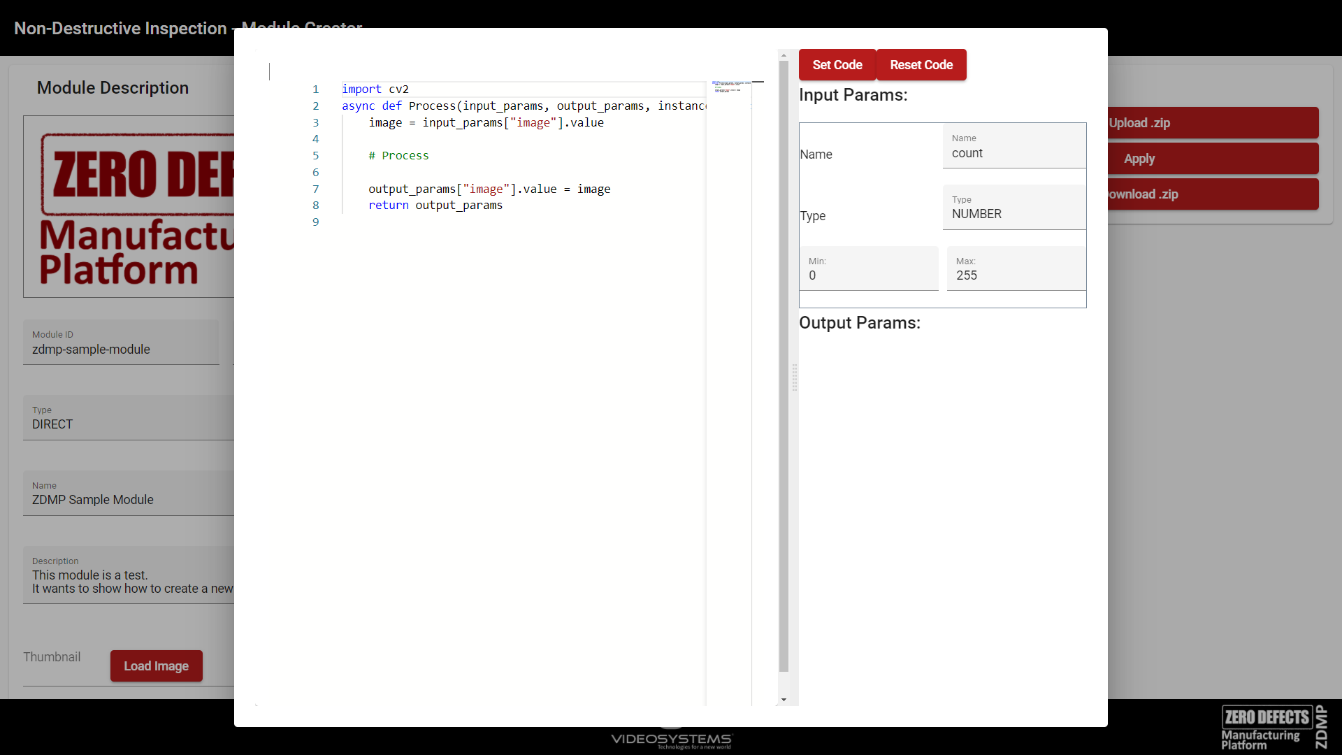
Figure 44. Module Creator – Function Code Editor
Function Tester
The Function Tester Dialog is used to test the function. This is the last step to check that the function is behaving as desired. The input parameters, on the left, must be set to run the process, which is executed by clicking on the Process button. On the right, the output parameters of the process are shown, with their relative value.
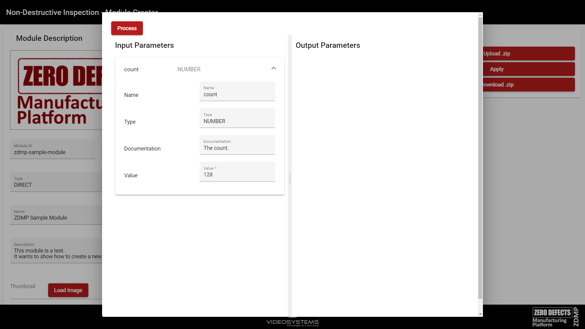
Figure 45. Crete Module – Function Tester
Apply Module
On the right side of Figure 39, there is the Apply Module controller.
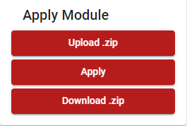
Figure 46. Module Creator – Apply Module controller
Upload .zip: Load a previously developed module to for further editing
Apply: Saves the configuration
Download .zip: Download the module to upload it to the Marketplace
Upload the module to the Marketplace
The .zip file must be uploaded to the Marketplace to appear in the Builder. A new product must then be created. Please check the Marketplace documentation for more information.
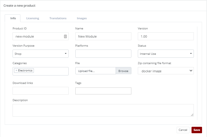
Figure 47. Marketplace – Create a new product
The .zip file must the uploaded by clicking Browse.
Develop an EXTERNAL_IMAGE Module
Instead of developing a module based on the Python programming language, users can develop an EXTERNAL_IMAGE module, which is based on a container to execute the module and its functions. Thanks to the containerization technology, it does not matter what programming language or libraries are used.
The flow to develop an EXTERNAL_IMAGE module can be summarized by the following chart:
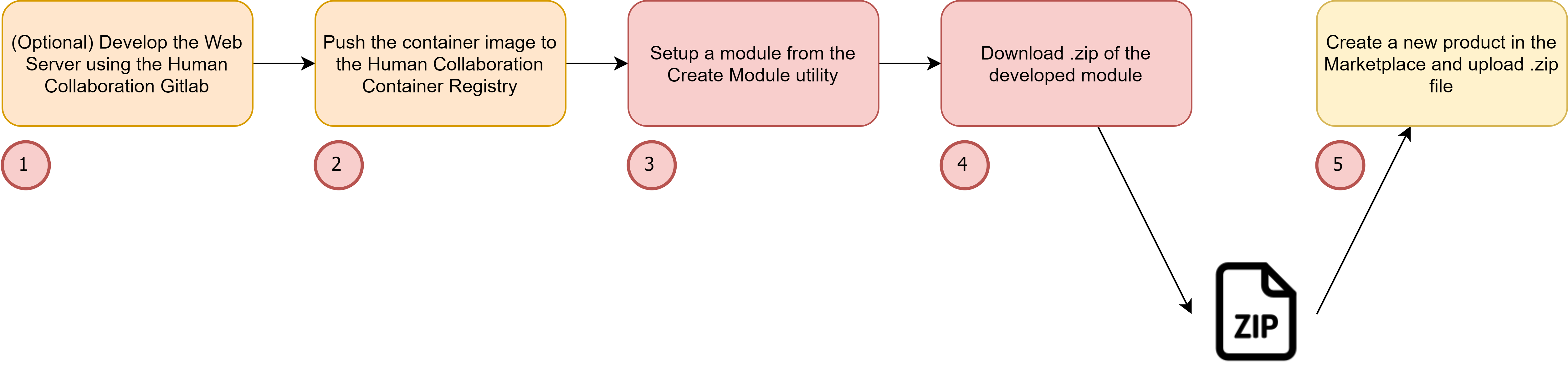
Figure 48. EXTERNAL_IMAGE development
To explain these steps, an example module is developed from start to finish. An AI Classification Inference module is developed, which allows classification of an image. It is based on TensorFlow, and it will use the trained model from this example. A function called “inference” is created, that has these input parameters:
model: The trained model
image: The image to classify
and these output parameters:
predicted_class: The predicted class
predictions: The probabilities per class
Develop the Web Server
The container must be a Web Server that exposes some endpoints to execute the processing on the module’s functions. The following endpoints must be exposed by the Web Server:
/, GET method, used for health check
/process, POST method, used to execute a process
The OpenAPI specification for the Web Server can be found here.
The /process endpoint receives this object:
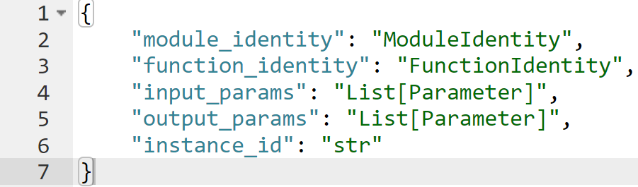
Figure 49. The /process request object
module_identity: Identifies the module, it can be ignored
function_identity: Contains the ID of the function of the process request
input_params: The input parameters of the process request
output_params: The default output parameters
instance_id: Unique ID of the process request
And it must respond with:
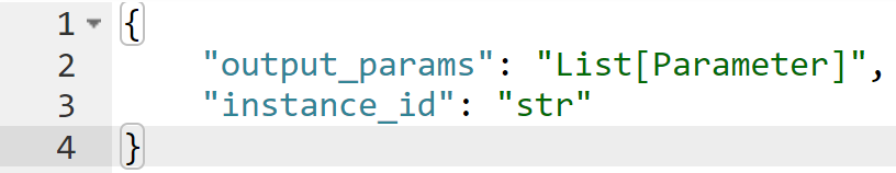
Figure 50. The /process response object
output_params: The processed output parameters
instance_id: Unique ID of the process request (same of the request)
Users can develop the Web Server on the Human Collaboration Gitlab. This way, it is easier to keep track of the developed modules in a centralized place and use CI/CD to automatically compile the container image. To create a new project in GitLab, create a new blank project.
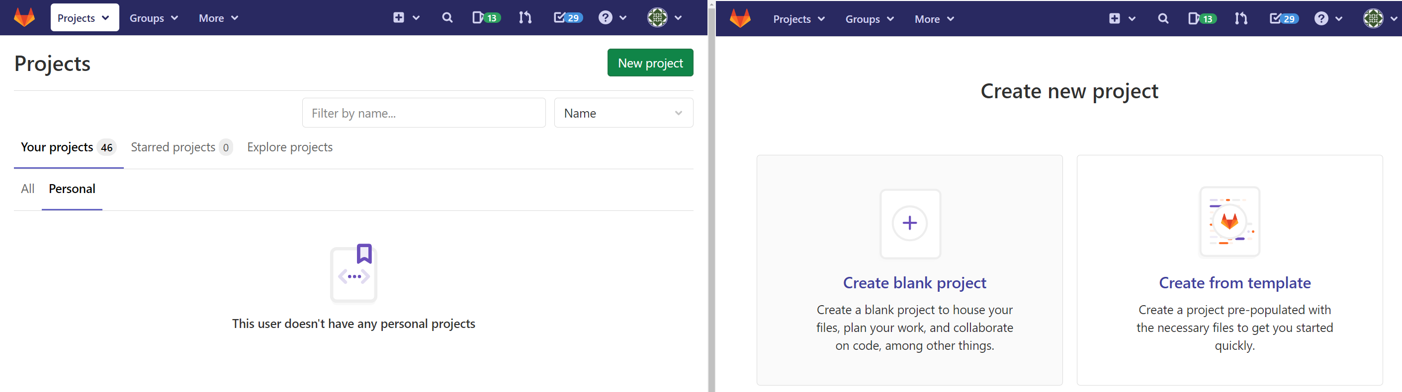
Figure 51. Human Collaboration Gitlab personal projects
The project name must be set, and the Project URL should point to the user for personal projects, or a group for shared projects.
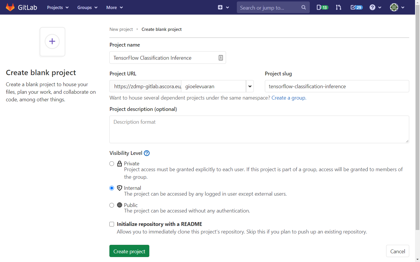
Figure 52. Human Collaboration GitLab create project
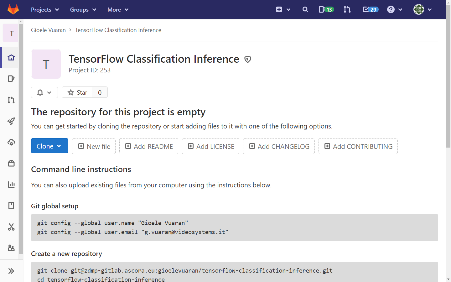
Figure 53. Human Collaboration GitLab project created correctly
Users can now clone the repository and develop the Web Server.
git clone ....
For this example, the Web Server is in Python with the help of the FastAPI library. Here is a link to the source code repository. This example is useful for understanding a typical scenario, and it can be used as a template for future projects.
In the app/main.py file, the HTTP endpoints are defined following the OpenAPI specification above. The models are defined in the models folder.
from fastapi import FastAPI
from deserializer import deserialize_parameter
from inference import run_inference
from models.process_request import ProcessRequest
from models.process_response import ProcessResponse

app = FastAPI()

@app.get("/")
def health_check():
    return

@app.post("/process", response_model=ProcessResponse)
def process(process_request: ProcessRequest):
    # Deserialize input & output parameters
    for input_param in process_request.input_params:
        deserialize_parameter(input_param, process_request.instance_id)
    for output_param in process_request.output_params:
        deserialize_parameter(output_param, process_request.instance_id)

    if(process_request.function_identity.function_id == "inference"): ...
    elif(process_request.function_identity.function_id == "...."): ...
Inside the body of the /process function the actual processing code must be inserted. The parameters, though, must be deserialized to be used, just like with the regular component APIs. Images and files require then particular attention. In the case of IMAGE and FILE parameters, the file_type field indicates how they have been serialized.
RAW_B64: The image or the file is encoded to a base64 string
FILESYSTEM_STORAGE: The image or the file is present in the internal filesystem
INTERNAL_SHARED_FILESYSTEM: The image or the file is present in a private, internal shared filesystem
Some environment variables have been set to indicate some mount points. The following table indicates the procedure to get the real path of an image or a file.
| file_type | Real path |
|---|---|
| FILESYSTEM_STORAGE | FILESYSTEM_STORAGE_PATH + parameter.value |
| INTERNAL_SHARED_FILESYSTEM | INTERNAL_FILESYSTEM_SHARED_PATH + instance_id + parameter.value |
In the deserializer.py file parameters are deserialized. In this case, images are loaded as PIL Images, which is a Python library. In this case, a PIL Image is required for Tensorflow, but in general there are no constraints. The library of choice can be used, like OpenCV, Scikit, etc, based on the needs of the application.
import base64
import io
import os

import PIL
import PIL.Image

from models.parameter import Parameter


def deserialize_image(parameter: Parameter, instance_id: str):
    if(parameter.file_type == "FILESYSTEM_STORAGE"):
        file_path = os.environ["FILESYSTEM_STORAGE_PATH"] + \
            "/" + parameter.value
        parameter.value = PIL.Image.open(file_path)
    elif(parameter.file_type == "INTERNAL_SHARED_FILESYSTEM"):
        file_path = os.environ["INTERNAL_FILESYSTEM_SHARED_PATH"] + \
            instance_id + "/" + parameter.value
        parameter.value = PIL.Image.open(file_path)
    elif(parameter.file_type == "RAW_B64"):
        buff = io.BytesIO(base64.b64decode(parameter.value))
        parameter.value = PIL.Image.open(buff)


def deserialize_file(parameter: Parameter, instance_id: str):
    if(parameter.file_type == "FILESYSTEM_STORAGE"):
        parameter.value = os.environ["FILESYSTEM_STORAGE_PATH"] + \
            "/" + parameter.value
    elif(parameter.file_type == "INTERNAL_SHARED_FILESYSTEM"):
        parameter.value = os.environ["INTERNAL_FILESYSTEM_SHARED_PATH"] + \
            instance_id + "/" + parameter.value


def deserialize_parameter(parameter: Parameter, instance_id: str):
    if(parameter.type == "IMAGE"):
        deserialize_image(parameter, instance_id)
    if(parameter.type == "FILE"):
        deserialize_file(parameter, instance_id)
After the deserialization, the processing can be performed. All the input parameters are ready to be used. The function_identity.function_id indicates which function to execute. A simple if statement is enough to decide which processing function to execute.
In the following image, there is the code of the function inference. The model and image parameter are retrieved, and a process is run by calling run_inference, which lives in another file for simplicity. The results of the run_inference function are copied in the output_params structure, and then the ProcessResponse object is returned.
if(process_request.function_identity.function_id == "inference"):
    # Get model and image parameters
    model_parameter = next(
        (input_param for input_param in process_request.input_params if input_param.name == "model"), None)
    image_parameter = next(
        (input_param for input_param in process_request.input_params if input_param.name == "image"), None)
    if(not model_parameter or not image_parameter):
        raise Exception("Invalid input parameters")

    # Run the inference
    predicted_class, predictions = run_inference(model_filename=model_parameter.value,
                                                    image=image_parameter.value)

    # Update ouput parameters
    predicted_class_parameter = next(
        (output_param for output_param in process_request.output_params if output_param.name == "predicted_class"), None)
    predictions_parameter = next(
        (output_param for output_param in process_request.output_params if output_param.name == "predictions"), None)
    predicted_class_parameter.value = predicted_class.item()
    predictions_parameter.value = predictions.tolist()[0]

    # Return the results
    return ProcessResponse(output_params=process_request.output_params, instance_id=process_request.instance_id)
This is all that is needed to develop a Web Server for an EXTERNAL_IMAGE module. The last step is to write a Dockerfile to create a container image. In the case of the example, this is quite simple.
FROM tensorflow/tensorflow

RUN pip install fastapi uvicorn

WORKDIR /app

COPY requirements.txt .
RUN pip install -r requirements.txt

COPY ./app /app
CMD ["uvicorn", "main:app", "--host", "0.0.0.0", "--port", "80"]
Push to the Container Registry
If the Web Server has been committed to the Human Collaboration GitLab, it is easier to use the CI/CD Pipelines to compile and push the container image to the Container Registry. In this case, the .gitlab-ci.yml file of the example repository is used.
If the code is hosted elsewhere, the image must be manually built and pushed to the Container Registry. In this case, a token with the “write_registry” scope must be created to be able to push the image.
The pushed container images can be viewed from the “Packages & Registries” menu on the left of the repository on GitLab.
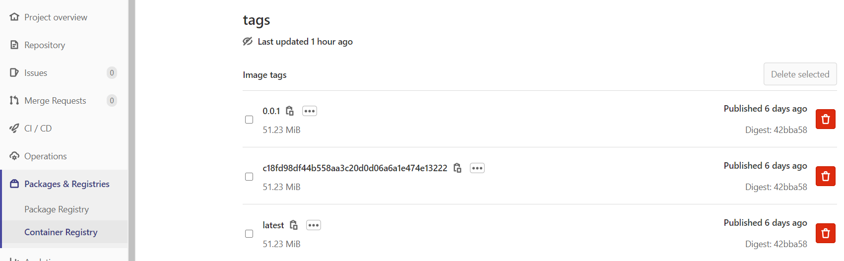
Figure 54. The GitLab Container Registry
Create the Module
Once the container image has been pushed, a new module must be created via the Module Creator utility. Following the example above, this should be filled in as per Figure 55. There a function inference has been added with its input and output parameters.
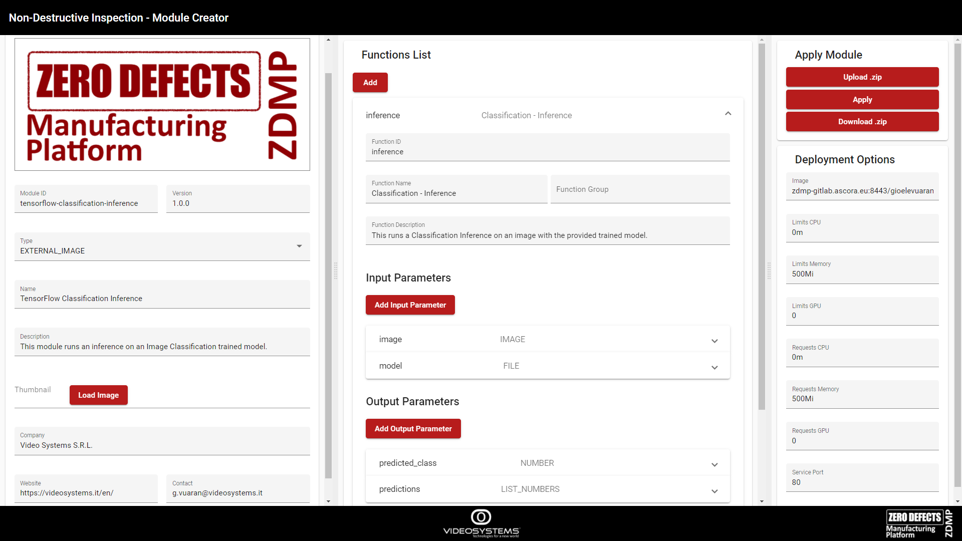
Figure 55. Module Creator filled with the example info
When the module type is set to EXTERNAL_IMAGE, the following menu will appear on the right.
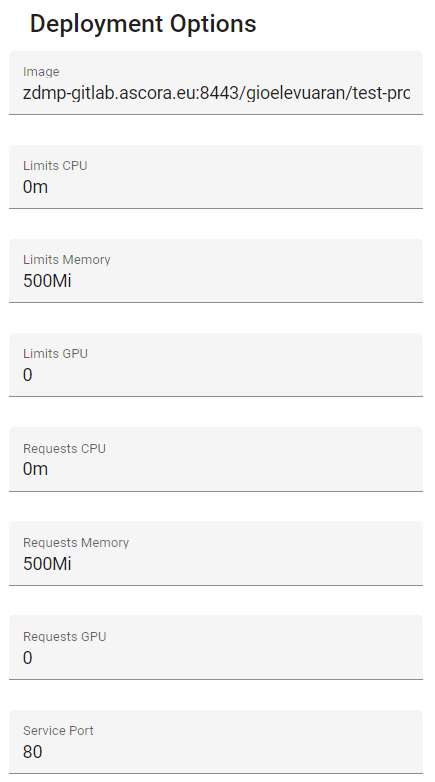
Figure 56. Deployment Options
Image: This is the container image tag. This can be retrieved from the Container Registry of Figure 54
Limits: These are the maximum resources to assign to the container (https://kubernetes.io/docs/concepts/configuration/manage-resources-containers/)
Requests: These are the minimum resources required for a container to start (https://kubernetes.io/docs/concepts/configuration/manage-resources-containers/)
Service Port: This is the port of the container to expose to access the web server
Use the Module
Once the module has been uploaded to the Marketplace and chosen in Builder, it can be used in the Designer. Here the input parameters are set:
model: The trained model of the example
image: An image to classify
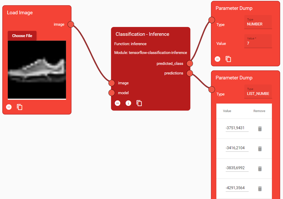
Figure 57. Inference function used in the Designer
Node-RED
The Component exposes APIs to make a processing. It can be difficult for a zApp, though, to continuously make requests to the Component and manage parameters.
Tools like Node-RED can be used to automate this. For example, it can be used to automatically call the Run Flow API when a new image from a camera is arrived.
Input and output parameters can be mapped to be set and dumped to Message Bus topics.
The Data Acquisition component has a Node-RED instance running.
The following schema shows a demo environment:
The Node-RED instance is connected to a camera
When new images arrive, the Run Flow API is called, with the image and various other parameters
The results parameters of the Run Flow API are sent to the Message Bus, so other components (zApps, Monitoring and Alerting, etc) can use them
The input parameters can be overwritten by the zApp using the Message Bus
Other ZDMP Components (like the Monitoring & Alerting) are listening to the Message Bus for messages
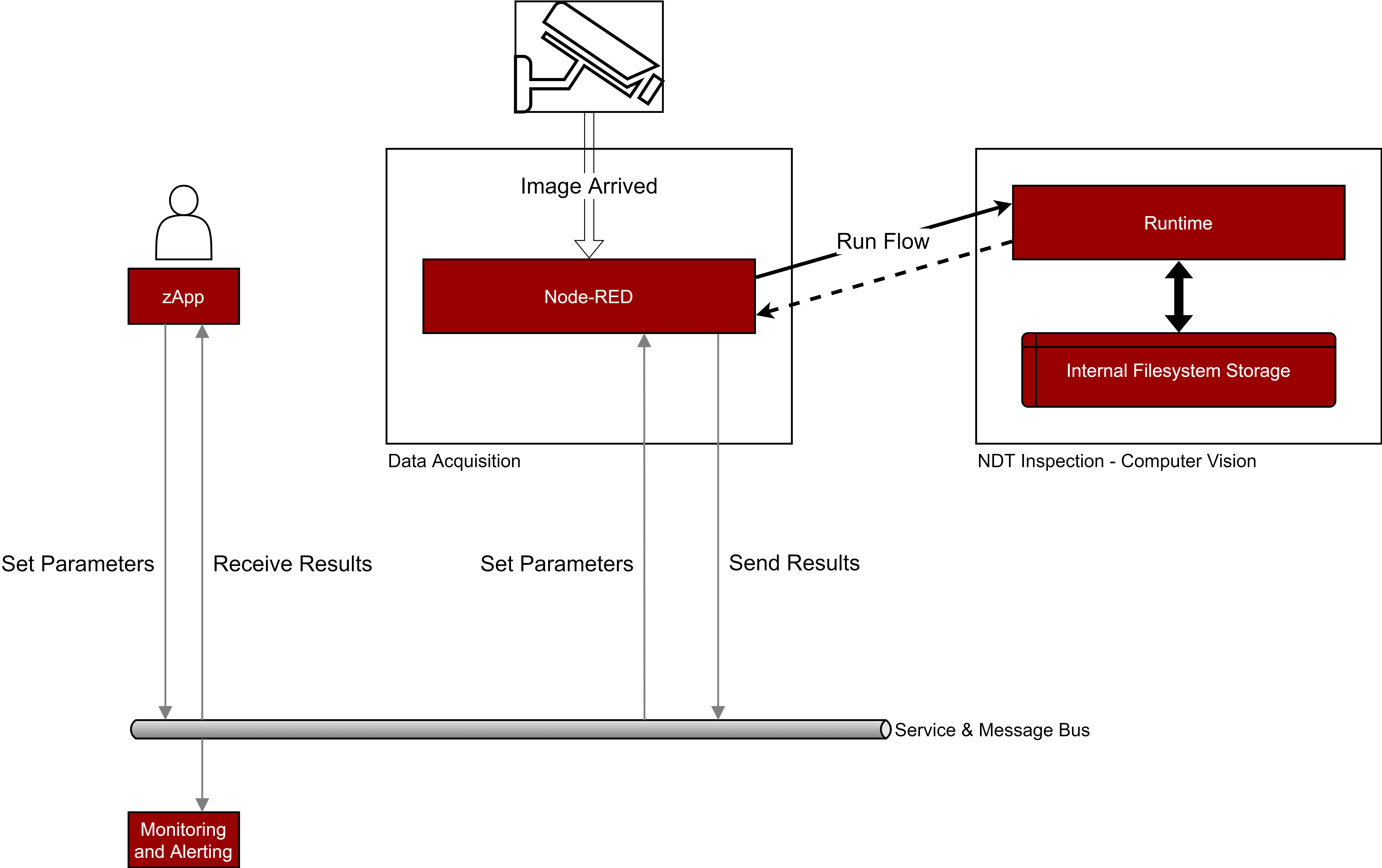
Figure 58. Example of a Node-RED orchestrated system
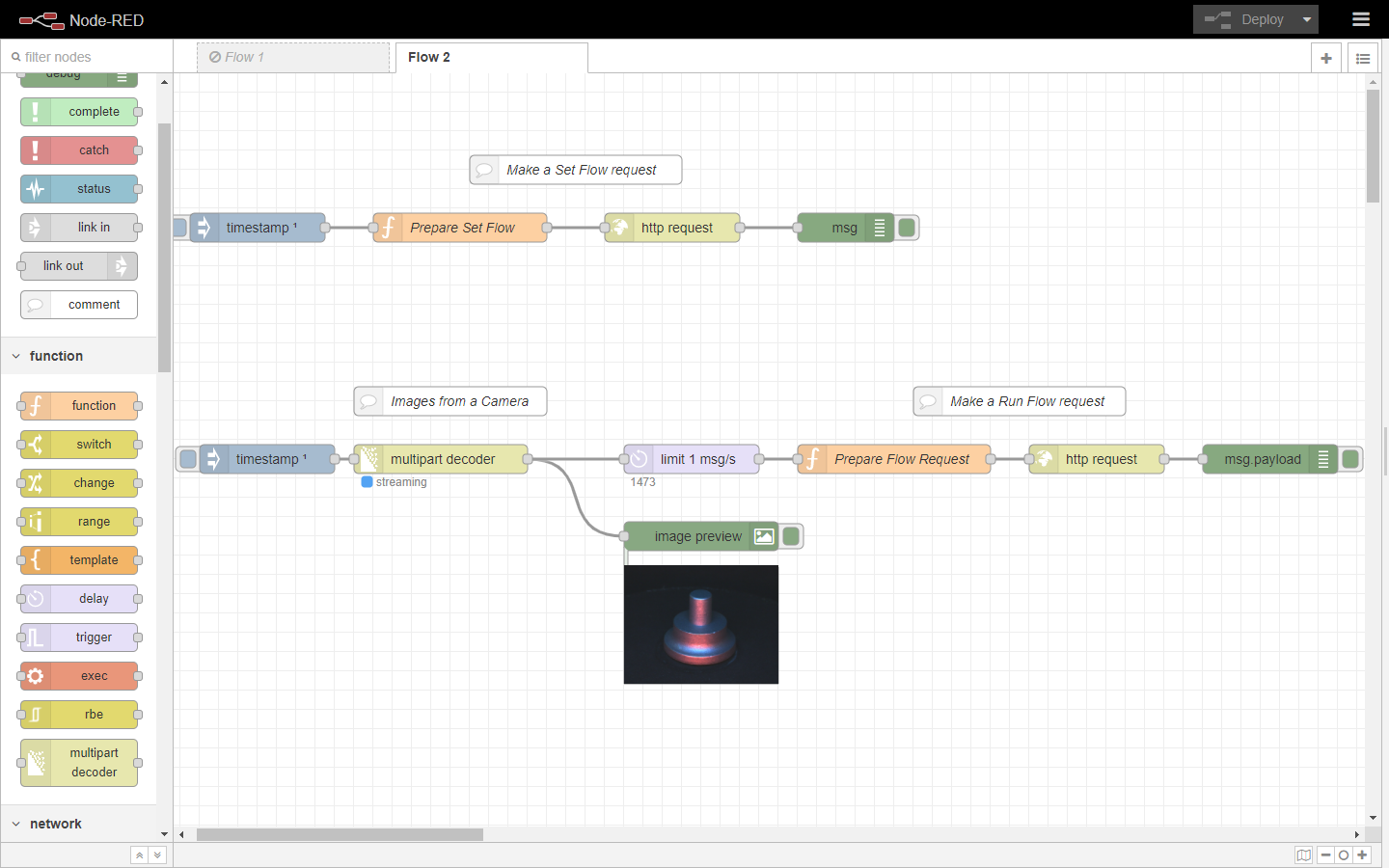
Figure 59. Example of a Node-RED flow